OLS Regression II

Agenda

• Two continuous variables
• One continuous & one categorical variable

Learning objectives

By the end of the lecture, you will be able to …

• Use R to produce multivariate regression
  
• Use R to create publication ready regression tables (e.g., Table 02)
  
• Understand the concept of modelling, interpreting, and visualizing interaction effects and marginal predictions.

Code-along 09

Download and open code-along-09.qmd

Packages

Load the standard packages and new package modelbased.

# install.packages("marginaleffects") # needed for modelbased
# install.packages("modelbased")

library(tidyverse) 
library(haven) # not core tidyverse
library(gssr)
library(gssrdoc)
library(summarytools)
library(gtsummary) 
library(moderndive)
library(modelbased)

Load your data

# Load all gss
data(gss_all)

Variables

• year Survey year
• tvhours Hours per day watching tv
• realrinc R’s income in constant $
• age Age of respondent
• educ Respondents highest edu credit
• hrs1 How many hours did you work last week
• childs How many children have you ever had?
• polviews Think of self as liberal or conservative
• sex Respondents sex
• marital R’s marital status

Make a df with only the (pretty) categorical and continuous variables we’ll analyze.

# Categorical Variables
my_cat <- gss_all |>
  select(id, year, polviews, sex, marital) |>
  zap_missing() |>
  mutate(
    polviews = as_factor(polviews),
    sex = as_factor(sex),
    marital = as_factor(marital)) |> 
  droplevels()

# Continuous Variables
my_con <- gss_all |>
  select(id, year, tvhours, age, educ, hrs1, realrinc, childs) |>
  mutate(
    age = as.numeric(age),
    educ = as.numeric(educ),
    hrs1 = as.numeric(hrs1),
    realrinc = as.numeric(realrinc),
    childs = as.numeric(childs))

# Combine the two dataframes
my_data <- full_join(my_cat, my_con, by = c("year", "id")) # match by 2 vars

Two continuous variables

Have the average number of children changed over time?

assumed to be a count, but can be modeled with OLS if treated as continuous

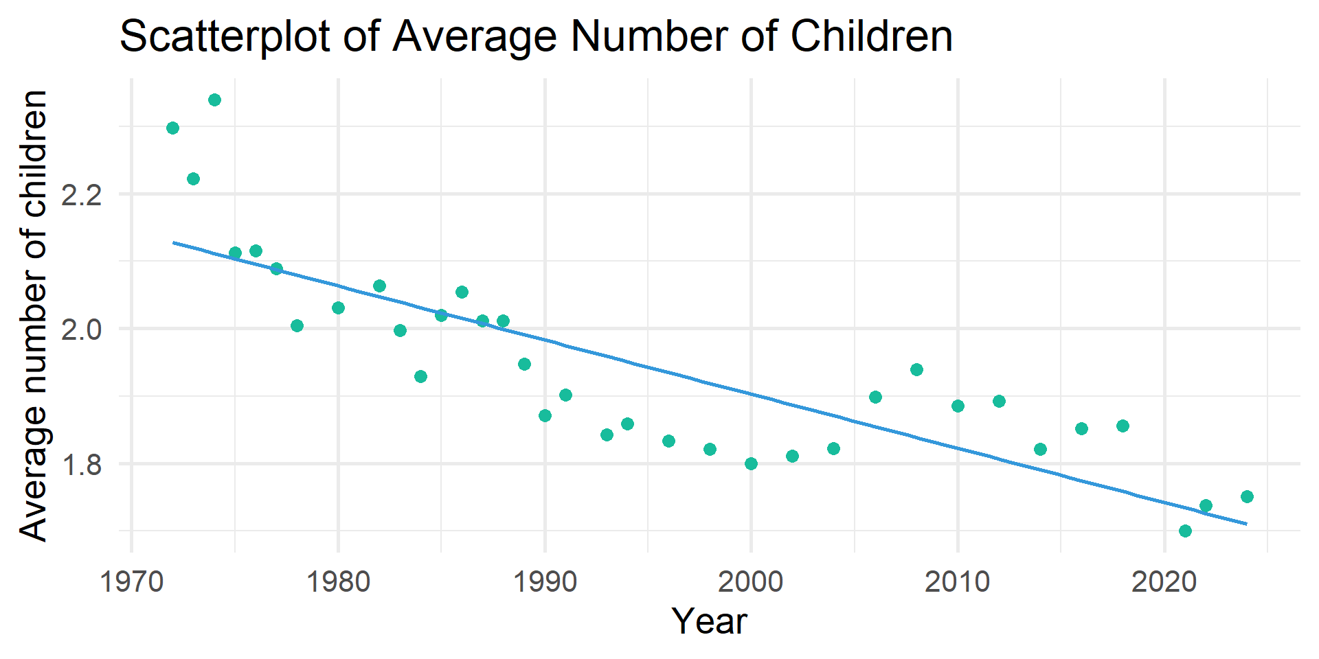
Simple Regression

model_01 <- lm(formula = childs ~ year, data = my_data)
get_regression_table(model_01)

# A tibble: 2 × 7
  term      estimate std_error statistic p_value lower_ci upper_ci
  <chr>        <dbl>     <dbl>     <dbl>   <dbl>    <dbl>    <dbl>
1 intercept   17.2       0.811      21.2       0   15.7     18.8  
2 year        -0.008     0         -18.9       0   -0.008   -0.007

PRE Measure

Get \(r^2\)

model_01 <- lm(formula = childs ~ year, data = my_data)
get_regression_summaries(model_01)

# A tibble: 1 × 9
  r_squared adj_r_squared   mse  rmse sigma statistic p_value    df  nobs
      <dbl>         <dbl> <dbl> <dbl> <dbl>     <dbl>   <dbl> <dbl> <dbl>
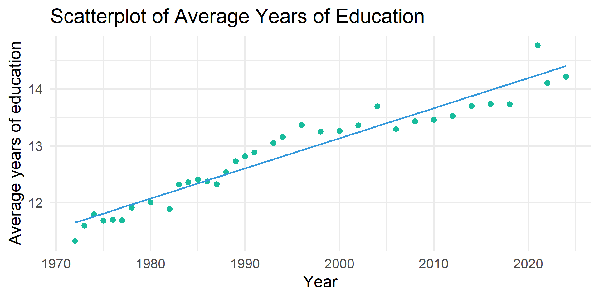
1     0.005         0.005  3.07  1.75  1.75      357.       0     1 75407

Are the trends explained by increases in education?

model_01 <- lm(formula = childs ~ year, data = my_data)
get_regression_table(model_01)

# A tibble: 2 × 7
  term      estimate std_error statistic p_value lower_ci upper_ci
  <chr>        <dbl>     <dbl>     <dbl>   <dbl>    <dbl>    <dbl>
1 intercept   17.2       0.811      21.2       0   15.7     18.8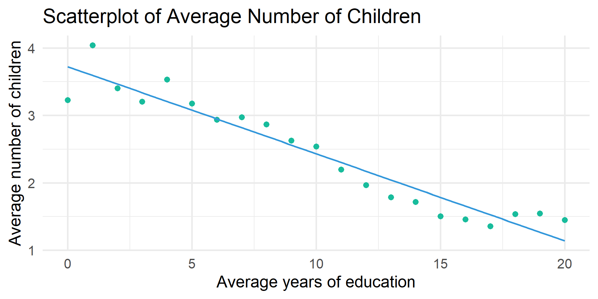  
2 year        -0.008     0         -18.9       0   -0.008   -0.007

model_02 <- lm(formula = childs ~ year + educ, data = my_data)
get_regression_table(model_02)

# A tibble: 3 × 7
  term      estimate std_error statistic p_value lower_ci upper_ci
  <chr>        <dbl>     <dbl>     <dbl>   <dbl>    <dbl>    <dbl>
1 intercept    5.26      0.813      6.47   0        3.66     6.85 
2 year        -0.001     0         -2.00   0.045   -0.002    0    
3 educ        -0.131     0.002    -64.5    0       -0.134   -0.127

Change in PRE Measure

get_regression_summaries(model_01)

# A tibble: 1 × 9
  r_squared adj_r_squared   mse  rmse sigma statistic p_value    df  nobs
      <dbl>         <dbl> <dbl> <dbl> <dbl>     <dbl>   <dbl> <dbl> <dbl>
1     0.005         0.005  3.07  1.75  1.75      357.       0     1 75407

get_regression_summaries(model_02)

# A tibble: 1 × 9
  r_squared adj_r_squared   mse  rmse sigma statistic p_value    df  nobs
      <dbl>         <dbl> <dbl> <dbl> <dbl>     <dbl>   <dbl> <dbl> <dbl>
1     0.057         0.057  2.90  1.70  1.70     2266.       0     2 75166

tbl_regression()

OLS Regression predicting number of children by survey year and years of education

model_02 |>
  tbl_regression(intercept = TRUE)  

Characteristic	Beta	95% CI	p-value
(Intercept)	5.3	3.7, 6.9	<0.001
GSS year for this respondent	0.00	0.00, 0.00	0.045
educ	-0.13	-0.13, -0.13	<0.001
Abbreviation: CI = Confidence Interval

model_02 |> tbl_regression(intercept = TRUE, estimate_fun = ~ style_number(.x, digits = 4))

tbl_regression()

OLS Regression predicting number of children by survey year and years of education

model_02 |>
  tbl_regression(
    intercept = TRUE) |>
  modify_column_hide(conf.low) |>
  modify_column_unhide(column = std.error) 

Characteristic	Beta	SE	p-value
(Intercept)	5.3	0.813	<0.001
GSS year for this respondent	0.00	0.000	0.045
educ	-0.13	0.002	<0.001
Abbreviations: CI = Confidence Interval, SE = Standard Error

tbl_regression()

OLS Regression predicting number of children by survey year and years of education

model_02 |>
  tbl_regression(
    intercept = TRUE) |>
  modify_column_hide(conf.low) |>
  modify_column_unhide(column = std.error) |>
  remove_abbreviation() |>
  add_significance_stars() |>
  add_glance_table(include = c("r.squared", "nobs"))

Characteristic	Beta1	SE
(Intercept)	5.3***	0.813
GSS year for this respondent	0.00*	0.000
educ	-0.13***	0.002
R²	0.057
No. Obs.	75,166
1 p<0.05; p<0.01; p<0.001

1 continuous variable & 1 categorical variable

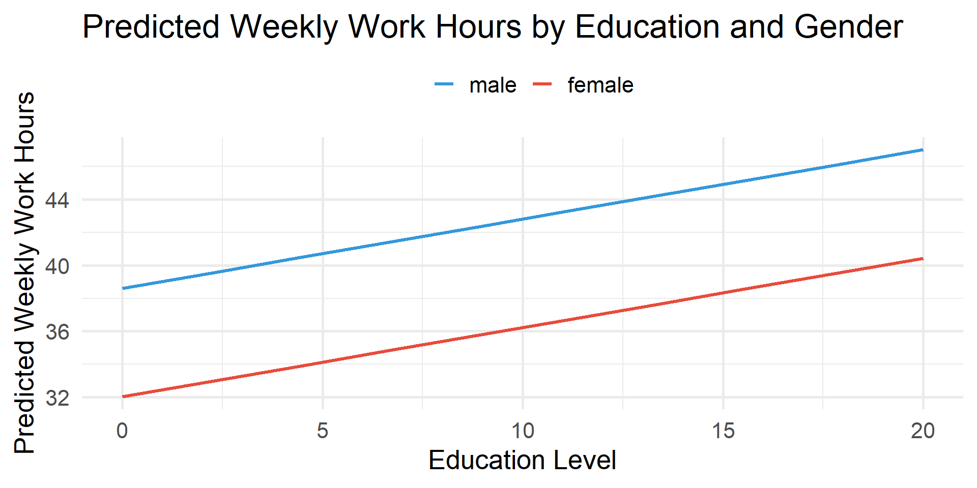
Are weekly hours worked related to education and gender?

model <- lm(hrs1 ~ educ + sex, data = my_data)

get_regression_table(model)

# A tibble: 3 × 7
  term        estimate std_error statistic p_value lower_ci upper_ci
  <chr>          <dbl>     <dbl>     <dbl>   <dbl>    <dbl>    <dbl>
1 intercept      38.6      0.32      121.        0   38.0     39.2  
2 educ            0.42     0.022      18.7       0    0.376    0.464
3 sex: female    -6.58     0.132     -49.9       0   -6.83    -6.32 

tbl_regression()

OLS Regression predicting weekly work hours by years of education and gender

model |>
  tbl_regression(
    intercept = TRUE) |>
  modify_column_hide(conf.low) |>
  modify_column_unhide(
    column = std.error) |>
  remove_abbreviation() |>
  add_significance_stars() |>
  add_glance_table(
    include = c("r.squared", "nobs"))

Characteristic	Beta1	SE
(Intercept)	39***	0.320
educ	0.42***	0.022
sex
male	—	—
female	-6.6***	0.132
R²	0.061
No. Obs.	43,167
1 p<0.05; p<0.01; p<0.001

tbl_regression()

OLS Regression predicting weekly work hours by years of education and gender

model |>
  tbl_regression(
    intercept = TRUE,
    show_single_row = sex,
    label = list(sex = "Women")) |>
  modify_column_hide(conf.low) |>
  modify_column_unhide(
    column = std.error) |>
  remove_abbreviation() |>
  add_significance_stars() |>
  add_glance_table(
    include = c("r.squared", "nobs"))

Characteristic	Beta1	SE
(Intercept)	39***	0.320
educ	0.42***	0.022
Women	-6.6***	0.132
R²	0.061
No. Obs.	43,167
1 p<0.05; p<0.01; p<0.001

estimate_means()

# Get predicted values
preds <- estimate_means(model, by = c("sex"))

# Preview the new df
preds |>
  as_tibble() |> 
  head()

# A tibble: 2 × 7
  sex     Mean     SE CI_low CI_high     t    df
  <fct>  <dbl>  <dbl>  <dbl>   <dbl> <dbl> <int>
1 male    44.4 0.0923   44.2    44.5  480. 43164
2 female  37.8 0.0939   37.6    38.0  402. 43164

R calculates the mean values of every variable in the model except sex, and sets all of those variables equal to their means. Then (once again) it sets female = 0 in every observation, calculates predicted probabilities for each individual, and averages those.

Then it goes back and resets female to 1 in every observation, again calculates predicted probabilities for each individual and outputs the average of those.

Outputs can be interpreted as the predicted probabilities for women and men if they were all average in all other respects.

estimate_means()

# Get predicted values
preds <- estimate_means(model, by = c("educ", "sex"))

# Preview the new df
preds |>
  as_tibble() |> 
  head()

estimate_means()

\(\color{#18bc9c}{38.601} + \color{#fd7e14}{0.420}_{educ} - \color{#e74c3c}{6.576}_{female}\)

# A tibble: 6 × 8
   educ sex     Mean    SE CI_low CI_high     t    df
  <dbl> <fct>  <dbl> <dbl>  <dbl>   <dbl> <dbl> <int>
1  0    male    38.6 0.320   38.0    39.2 121.  43164
2  0    female  32.0 0.323   31.4    32.7  99.0 43164
3  2.22 male    39.5 0.273   39.0    40.1 145.  43164
4  2.22 female  33.0 0.276   32.4    33.5 119.  43164
5  4.44 male    40.5 0.226   40.0    40.9 179.  43164
6  4.44 female  33.9 0.230   33.4    34.3 148.  43164

men with 0 years of education = \(\color{#18bc9c}{38.601} + \color{#fd7e14}{0.420}_{educ}*0\)
women with 0 years of education \(\color{#18bc9c}{38.601} + \color{#fd7e14}{0.420}_{educ}*0 -\color{#e74c3c}{6.576}_{female}\)
men with 2.222 years of education \(\color{#18bc9c}{38.601} + \color{#fd7e14}{0.420}_{educ}*2.222\)
women with 2.222 years of education \(\color{#18bc9c}{38.601} + \color{#fd7e14}{0.420}_{educ}*2.222-\color{#e74c3c}{6.576}_{female}\)

# Plot using ggplot2
preds |>
  ggplot(aes(x = educ, y = Mean, color = sex)) +
    geom_line(linewidth = 1.2) +
    labs(
      title = "Predicted Weekly Work Hours by Education and Gender",
      x = "Education Level",
      y = "Predicted Weekly Work Hours",
      color = " ") +
    theme_minimal(20) +
    theme(legend.position = "top")

Are weekly hours worked related to education and marital status?

model <- lm(hrs1 ~ educ + marital, data = my_data)
get_regression_table(model)

# A tibble: 6 × 7
  term                   estimate std_error statistic p_value lower_ci upper_ci
  <chr>                     <dbl>     <dbl>     <dbl>   <dbl>    <dbl>    <dbl>
1 intercept                36.5       0.33    110.      0       35.9     37.1  
2 educ                      0.378     0.023    16.4     0        0.333    0.424
3 marital: widowed         -5.94      0.385   -15.4     0       -6.70    -5.19 
4 marital: divorced         0.605     0.198     3.06    0.002    0.218    0.993
5 marital: separated       -0.278     0.379    -0.733   0.464   -1.02     0.465
6 marital: never married   -1.76      0.163   -10.8     0       -2.08    -1.44 

Regression Predicting Weekly Work Hours by Years of Education and Marital Status

model |>
  tbl_regression(
    intercept = TRUE,
    label = list(
      marital = "Marital status (ref. = married)")) |>
  remove_row_type(type = c("reference")) |>  
  modify_column_hide(conf.low) |>
  modify_column_unhide(
    column = std.error) |>
  remove_abbreviation() |>
  add_significance_stars() |>
  add_glance_table(
    include = c("r.squared", "nobs"))

Characteristic	Beta1	SE
(Intercept)	37***	0.330
educ	0.38***	0.023
Marital status (ref. = married)
widowed	-5.9***	0.385
divorced	0.61**	0.198
separated	-0.28	0.379
never married	-1.8***	0.163
R²	0.015
No. Obs.	43,178
1 p<0.05; p<0.01; p<0.001

Are daily TV hours related to education and political identity?

my_data <- my_data %>%
  mutate(pol_group = case_when(
    polviews %in% c("extremely liberal", "liberal", "slightly liberal") ~ "Liberal",
    polviews == "moderate, middle of the road" ~ "Moderate",
    polviews %in% c("slightly conservative", "conservative", "extremely conservative") ~ "Conservative",
    TRUE ~ NA_character_))

model <- lm(tvhours ~ educ + pol_group, data = my_data)

get_regression_table(model)

# A tibble: 4 × 7
  term                estimate std_error statistic p_value lower_ci upper_ci
  <chr>                  <dbl>     <dbl>     <dbl>   <dbl>    <dbl>    <dbl>
1 intercept              5.00      0.056     89.1        0    4.89     5.12 
2 educ                  -0.159     0.004    -40.4        0   -0.166   -0.151
3 pol_group: Liberal     0.157     0.031      5.15       0    0.097    0.217
4 pol_group: Moderate    0.192     0.028      6.76       0    0.136    0.247

relevel()

# Relevel pol_group so "Moderate" is the reference
my_data$pol_group <- relevel(factor(my_data$pol_group), 
                            ref = "Moderate")

model <- lm(tvhours ~ educ + pol_group, data = my_data)
get_regression_table(model)

# A tibble: 4 × 7
  term                    estimate std_error statistic p_value lower_ci upper_ci
  <chr>                      <dbl>     <dbl>     <dbl>   <dbl>    <dbl>    <dbl>
1 intercept                  5.20      0.054     96.4     0       5.09     5.30 
2 educ                      -0.159     0.004    -40.4     0      -0.166   -0.151
3 pol_group: Conservative   -0.192     0.028     -6.76    0      -0.247   -0.136
4 pol_group: Liberal        -0.035     0.03      -1.15    0.25   -0.093    0.024

Does the relationship between TV hours and education differ by political identity?

model <- lm(tvhours ~ educ * pol_group, data = my_data)

get_regression_table(model)

# A tibble: 6 × 7
  term                    estimate std_error statistic p_value lower_ci upper_ci
  <chr>                      <dbl>     <dbl>     <dbl>   <dbl>    <dbl>    <dbl>
1 intercept                  4.98      0.088    56.5     0        4.81     5.16 
2 educ                      -0.142     0.007   -21.1     0       -0.155   -0.129
3 pol_group: Conservative   -0.1       0.128    -0.781   0.435   -0.351    0.151
4 pol_group: Liberal         0.553     0.132     4.20    0        0.295    0.811
5 educ:pol_groupConserva…   -0.008     0.01     -0.787   0.431   -0.026    0.011
6 educ:pol_groupLiberal     -0.044     0.01     -4.55    0       -0.063   -0.025

The coefficient for educ is $-0.142 $, meaning that for moderates (the reference group), each additional year of education is associated with -0.142 fewer tv hours per day.

The coefficient for pol_group: Conservative is \(-0.1\). This is the difference in the outcome between moderates and conservatives when education = 0. Conservatives watch -0.1 TV hours per day fewer than moderates when education is zero. Not statistically significantly different.

The interaction term educ:pol_groupConservative is \(-0.008\). It tells us whether the relationship between education and TV hours differs between moderates and conservatives It adjusts the slope of education for conservatives So for conservatives, the effect of education is:

\(-0.142 -0.008 = -0.15\)

This means that for conservatives, each additional unit of education is associated with only \(-0.15\) fewer daily TV hours.

# Get predicted values
preds <- estimate_means(model, by = c("educ", "pol_group"))

# Plot using ggplot2
preds |>
  ggplot(aes(x = educ, y = Mean, color = pol_group)) +
    geom_line(linewidth = 1.2) +
    labs(
      title = "Predicted Daily TV Hours by Education and Political Identity",
      x = "Education Level",
      y = "Predicted TV Hours",
      color = "Political Identity") +
    theme_minimal(20) +
    theme(legend.position = "top")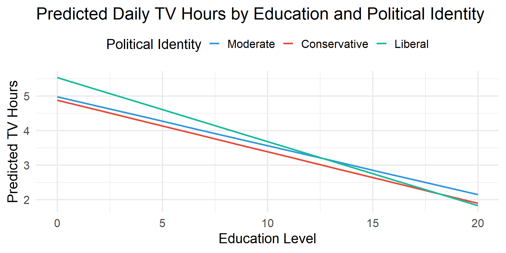

Think Like a Statistician

Think Like a Statistician

1. Run and interpret a regression predicting realrinc with hrs1 and educ

model <- lm(realrinc ~ hrs1 + educ, data = my_data)
get_regression_table(model)

# A tibble: 3 × 7
  term      estimate std_error statistic p_value lower_ci upper_ci
  <chr>        <dbl>     <dbl>     <dbl>   <dbl>    <dbl>    <dbl>
1 intercept  -33065.     802.      -41.2       0  -34637.  -31494.
2 hrs1          481.      10.5      45.6       0     460.     501.
3 educ         2746.      50.4      54.5       0    2647.    2845.

Think Like a Statistician

2. Add childs to the regression. Interpret the output.

model <- lm(formula = realrinc ~ hrs1 + educ + childs, data = my_data)
get_regression_table(model)

# A tibble: 4 × 7
  term      estimate std_error statistic p_value lower_ci upper_ci
  <chr>        <dbl>     <dbl>     <dbl>   <dbl>    <dbl>    <dbl>
1 intercept  -39248.     851.      -46.1       0  -40917.  -37580.
2 hrs1          481.      10.5      45.8       0     460.     501.
3 educ         2959.      51.2      57.8       0    2858.    3059.
4 childs       1960.      93.9      20.9       0    1776.    2144.

Think Like a Statistician

3. Add marital to the regression. Interpret the output.

model <- lm(formula = realrinc ~ hrs1 + educ + childs + marital, data = my_data)
get_regression_table(model)

# A tibble: 8 × 7
  term                   estimate std_error statistic p_value lower_ci upper_ci
  <chr>                     <dbl>     <dbl>     <dbl>   <dbl>    <dbl>    <dbl>
1 intercept               -33122.     886.     -37.4        0  -34859.  -31385.
2 hrs1                       468.      10.5     44.7        0     448.     489.
3 educ                      2888.      51.0     56.6        0    2788.    2988.
4 childs                    1021.     105.       9.76       0     816.    1226.
5 marital: widowed         -4122.     826.      -4.99       0   -5740.   -2503.
6 marital: divorced        -4029.     420.      -9.60       0   -4851.   -3206.
7 marital: separated       -5769.     816.      -7.07       0   -7368.   -4171.
8 marital: never married   -8792.     394.     -22.3        0   -9564.   -8020.