Bivariate Regression

Agenda

• Simple regression
• Categorical IV
• \(R^2\)

Learning objectives

By the end of the lecture, you will be able to …

• Use R to produce bivariate regression
• Use R to produce \(R^2\)

Code-along 08

Download and open code-along-08.qmd

Packages

Load the standard packages & new package moderndive

# install.packages(broom.helpers) # needed for moderndive
# install.packages("moderndive")

library(tidyverse) 
library(haven) # not core tidyverse
library(summarytools)
library(gtsummary) 
library(moderndive)

Simple Regression

Simple Regression

Regression and correlation are ways to identify whether two interval-ratio variables are statistically dependent

as the value of one variable changes, the other also tends to change

Code Meets Question

What is the relationship between literacy rate and rate of tertiary education?

literacy rate
% of adult population that is literate

rate of tertiary education
the % of students enrolled/eligible within the age range

Example df

# Create columns
literacy <- c(31.7, 79.3, 85.4, 41.0, 54.7, 97.9, 92.8, 67.1, 97.8, 60.4, 87.5, 99.1)
educ <- c(3.74, 10.4, 20.4, 4.46, 9.53, 78.6, 31.5, 16.2, 65.8, 10.3, 30.8, 40.1)

# Combine into a data frame
df <- data.frame(literacy, educ)

# View the data frame
print(df)

   literacy  educ
1      31.7  3.74
2      79.3 10.40
3      85.4 20.40
4      41.0  4.46
5      54.7  9.53
6      97.9 78.60
7      92.8 31.50
8      67.1 16.20
9      97.8 65.80
10     60.4 10.30
11     87.5 30.80
12     99.1 40.10

tidy_summary()

moderndive::tidy_summary() returns commonly used summary statistics in a tidy format.

df |>
  tidy_summary()

# A tibble: 2 × 11
  column       n group type      min    Q1  mean median    Q3   max    sd
  <chr>    <int> <chr> <chr>   <dbl> <dbl> <dbl>  <dbl> <dbl> <dbl> <dbl>
1 literacy    12 <NA>  numeric 31.7   59.0  74.6   82.4  94.0  99.1  23.2
2 educ        12 <NA>  numeric  3.74  10.1  26.8   18.3  33.6  78.6  24.2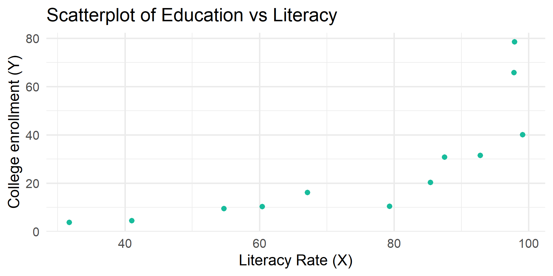

# Create scatterplot
df |>
  ggplot(aes(x = literacy, y = educ)) +
  geom_point(color = "#18BC9C", size = 3) +
  labs(
    title = "Scatterplot of Education vs Literacy",
    x = "Literacy Rate (X)",
      y = "College enrollment (Y)"
  ) +
  theme_minimal(20)

Linear relationship

When two interval-ratio level variables are related to one another we can approximate the relationship by drawing a straight line through the center of the observations on the scatterplot.

A bivariate regression analysis finds the best possible line to summarize the observed relationship between X and Y

# Create scatterplot with regression line
df |>
  ggplot(aes(x = literacy, y = educ)) +
    geom_point(color = "#18BC9C", size = 3) +
    geom_smooth(method = "lm", se = FALSE, color = "#3498DB") +
    labs(
      title = "Scatterplot of Education vs Literacy with Regression Line",
      x = "Literacy Rate (X)",
      y = "College enrollment (Y)"
    ) +
    theme_minimal(20)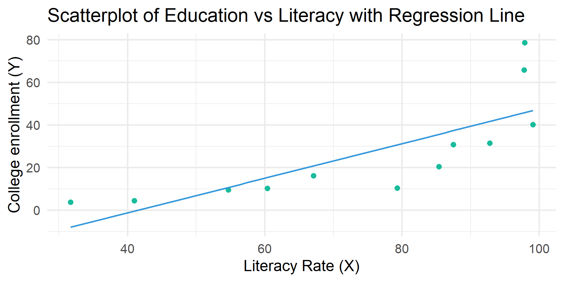

\(\hat{y} = a + bX\)

\(\hat{y}\) = the predicted score on the dependent variable

\(X\) = the score on the independent variable

\(a\) = the Y-intercept, or the point where the line crosses the Y-axis (\(a\) is the value of \(Y\) when \(X\) is equal to 0).

\(b\) = the slope of the regression line, or the change in \(Y\) for each unit of change in \(X\).

\(\hat{y} = a + bX\)

Positive relationship
When \(b\) is positive, then when \(X\) increases, \(\hat{y}\) increases

Negative relationship
When \(b\) is negative, then when \(X\) increases, \(\hat{y}\) decreases

With relationships that are imperfect, we must fit the best available line to represent the data.

ASK: Would \(b\) be positive or negative? What about \(a\)?

\(\hat{y} = a + bX\)

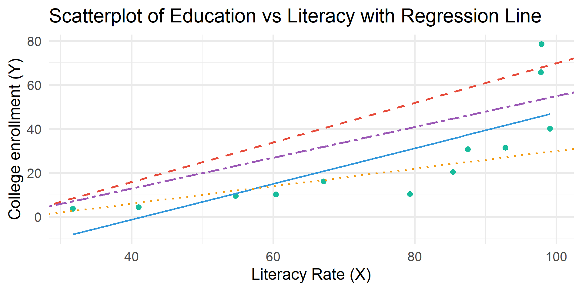
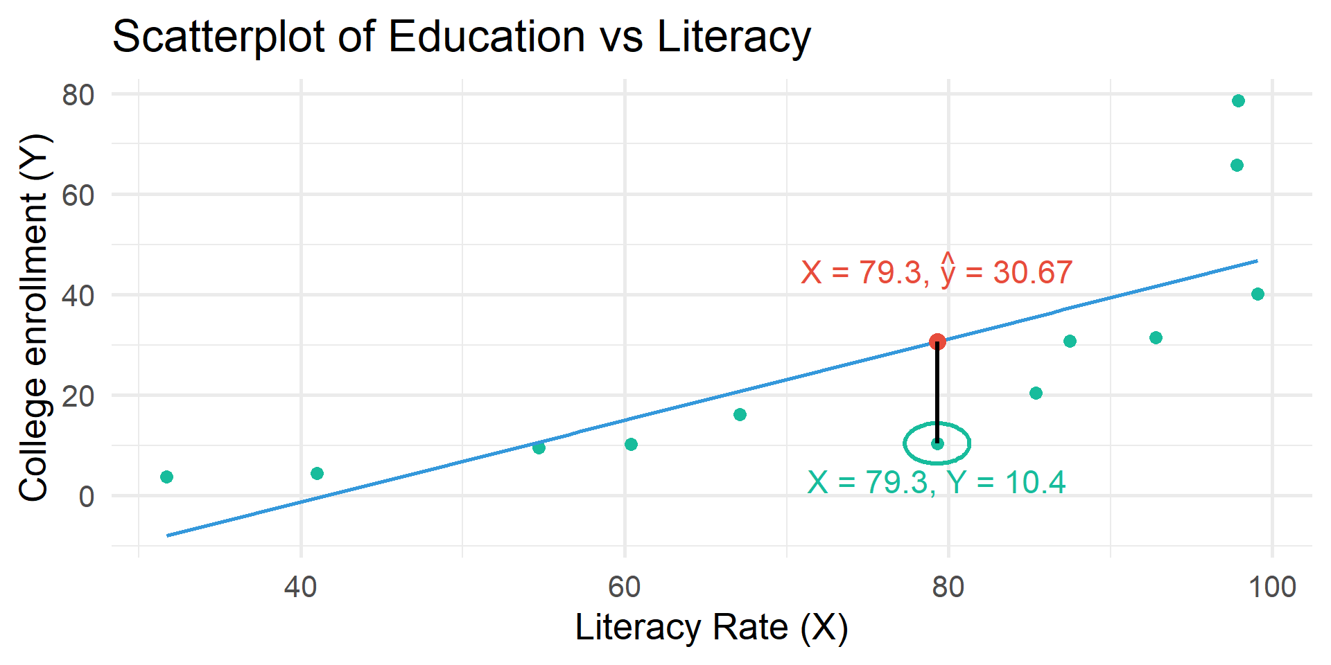
Regression finds the best fitting line that goes through the data with the least distance (error) between all points and the line.

AKA the “least squares line” referring to the least amount of squared error.

\(\hat{y}\) is the predicted value of the dependent variable, based on a given value of the independent variable.

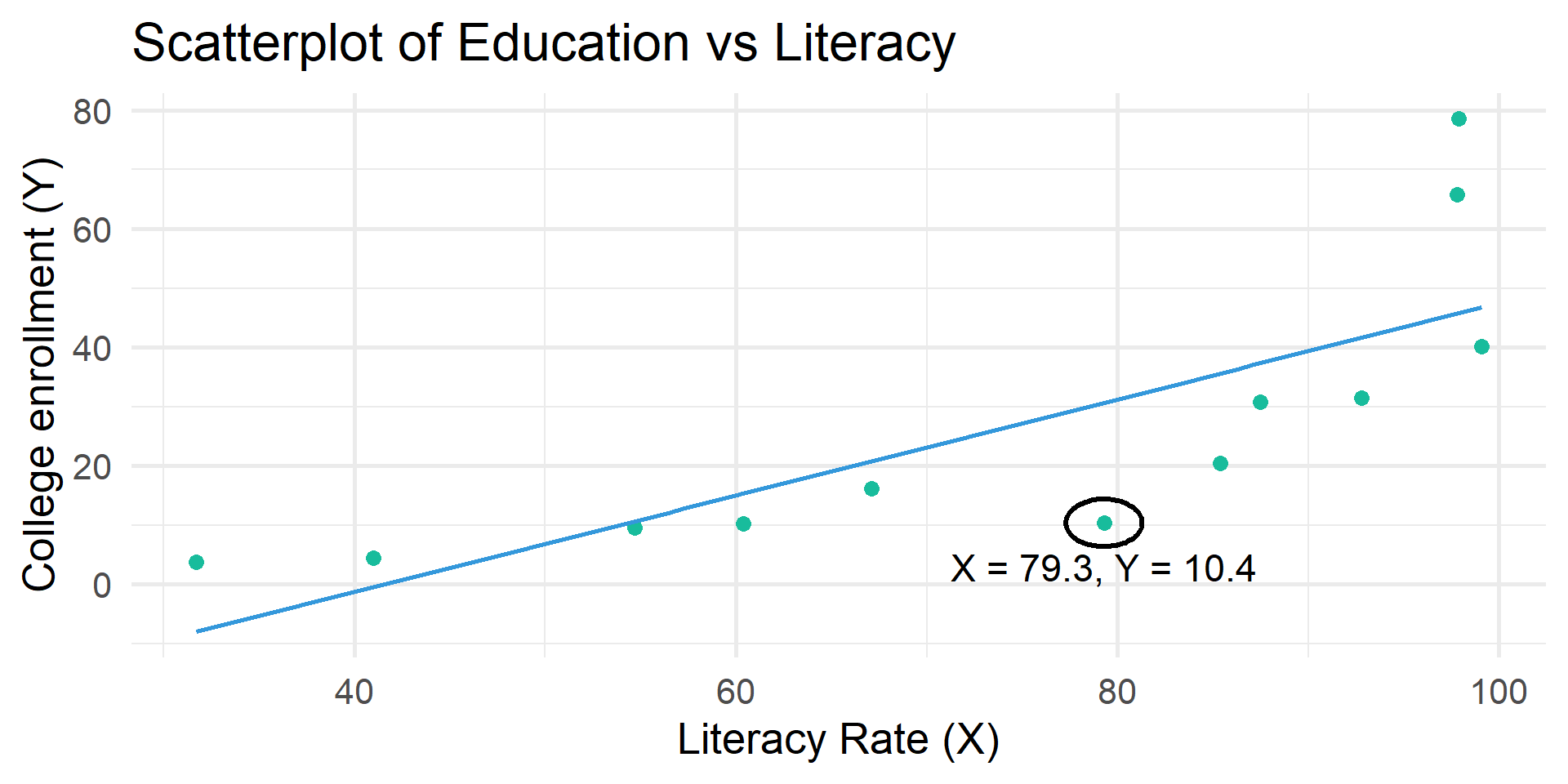
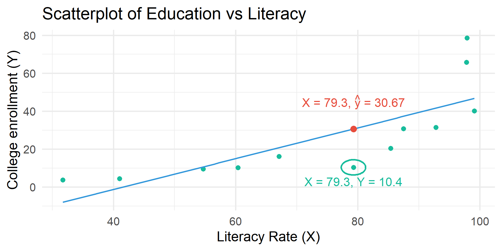
Residual = error (\(e\))

Calculated based on the difference between \(Y\) and \(\hat{y}\)

\(Y\) = observed value of \(Y\) for given value of \(X\)

\(\hat{y}\) = predicted value of \(Y\) for given value of \(X\)

Residual table

literacy	educ	educ_hat	residual
31.7	3.74	-7.995	11.735
79.3	10.40	30.671	-20.271
85.4	20.40	35.626	-15.226
41.0	4.46	-0.440	4.900
54.7	9.53	10.688	-1.158
97.9	78.60	45.780	32.820

OLS Regression

\(\hat{y} = a + bX\)

Least-squares line
The line where the residual sum of squares is at a minimum

Ordinary least-squares (OLS) regression
The statistical technique that produces the least-squares line Sometimes referred to as linear regression

\(\hat{y} = a + bX\)

Calculus demonstrates the formula for \(b\) and \(a\) will result in a regression line that minimizes the sum of squares.

Run a regression model.

lm(educ ~ literacy, data = df)

Call:
lm(formula = educ ~ literacy, data = df)

Coefficients:
(Intercept)     literacy  
   -33.7449       0.8123  

\(\hat{y} = -33.75 + .81X\)

\(\hat{y} = -33.75 + .81X\)

When the literacy rate in a country is 0, the college enrollment rate is predicted to be -33.57 (\(a\))

For every one unit increase in the literacy rate, the college enrollment rate is expected to rise by 0.81 (\(b\))

Is this statistically significant?

cor.test()

Run and interpret the correlation for educ and literacy.

cor.test(
     ~ educ + literacy,
     data = df,
     method = "pearson",
     na.action = na.omit
 ) 

    Pearson's product-moment correlation

data:  educ and literacy
t = 3.942, df = 10, p-value = 0.002766
alternative hypothesis: true correlation is not equal to 0
95 percent confidence interval:
 0.3731885 0.9352545
sample estimates:
      cor 
0.7800287 

There is a strong, positive association between the literacy rate and enrollment in tertiary education among nations.

get_regression_table()

model <- lm(educ ~ literacy, data = df)

get_regression_table(model)

# A tibble: 2 × 7
  term      estimate std_error statistic p_value lower_ci upper_ci
  <chr>        <dbl>     <dbl>     <dbl>   <dbl>    <dbl>    <dbl>
1 intercept  -33.7      16.0       -2.10   0.062  -69.5       1.98
2 literacy     0.812     0.206      3.94   0.003    0.353     1.27

statistic Test whether the coefficient is different from 0. Get the t-values by dividing the estimate by its standard error.

p-value Two-tail p-values for the test statistic

The p value is the same for correlation and simple regression.

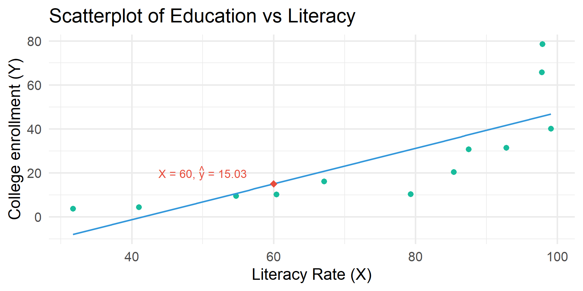
Prediction

\(\hat{y} = -33.75 + .81X\)

A regression equation can also be used to create predicted Y values for each value of X

If X = 60, \(Y\) is predicted to be:

\(\hat{y} = -33.75 + .81(60)\)
\(\hat{y} = -33.75 + 48.6\)
\(\hat{y} = 15.03\)

Categorical IV

Add a categorical variable

# Use mutate and case_when to add the country_group column
df <- df %>%
  mutate(country_group = case_when(
    literacy < 50 ~ "Low Literacy",
    literacy >= 50 & literacy <= 80 ~ "Medium Literacy",
    literacy > 80 ~ "High Literacy"
  ))

head(df)

  literacy  educ   country_group
1     31.7  3.74    Low Literacy
2     79.3 10.40 Medium Literacy
3     85.4 20.40   High Literacy
4     41.0  4.46    Low Literacy
5     54.7  9.53 Medium Literacy
6     97.9 78.60   High Literacy

get_regression_table()

model_2 <- lm(educ ~ country_group, data = df)

get_regression_table(model_2)

# A tibble: 3 × 7
  term                    estimate std_error statistic p_value lower_ci upper_ci
  <chr>                      <dbl>     <dbl>     <dbl>   <dbl>    <dbl>    <dbl>
1 intercept                   44.5      6.94      6.42   0         28.8    60.2 
2 country_group: Low Lit…    -40.4     13.9      -2.91   0.017    -71.8    -9.03
3 country_group: Medium …    -32.9     11.0      -3      0.015    -57.8    -8.10

What does the intercept mean? Which group has the smallest proportion of college enrolles? Is it statistically significantly different (than what group?)? What proportion is enrolled in college in low literacy countries? medium literacy?

\(R^2\)

Proportional Reduction of Error

The better a least-squares line is, the better it can predict an outcome with the least amount of error

\(r^2\) is a proportional reduction of error (PRE) measure

\(PRE = \frac{E1 - E2}{E1}\)

It tells us how well the regression model fits the data

\(PRE = \frac{E1 - E2}{E1}\)

E1
Errors of prediction made when IV is ignored

Equivalent to the sum of errors we would have if we guessed that every Y was equal to the mean of Y

aka Sum of Squares Total (SST)

E2
Errors of prediction made based on IV

Equivalent to the sum of errors we would have if we used our least squares line to predict Y

aka Sum of Squared Errors (SSE)

Use get_regression_points() to see the residuals.

model <- lm(educ ~ literacy, data = df)

get_regression_points(model)

# A tibble: 12 × 5
      ID  educ literacy educ_hat residual
   <int> <dbl>    <dbl>    <dbl>    <dbl>
 1     1  3.74     31.7    -8.00    11.7 
 2     2 10.4      79.3    30.7    -20.3 
 3     3 20.4      85.4    35.6    -15.2 
 4     4  4.46     41      -0.44     4.9 
 5     5  9.53     54.7    10.7     -1.16
 6     6 78.6      97.9    45.8     32.8 
 7     7 31.5      92.8    41.6    -10.1 
 8     8 16.2      67.1    20.8     -4.56
 9     9 65.8      97.8    45.7     20.1 
10    10 10.3      60.4    15.3     -5.02
11    11 30.8      87.5    37.3     -6.53
12    12 40.1      99.1    46.8     -6.65

\(R^2\) ranges from 0 to 1.0

1.0 = Our independent variable accounts for all the variation that we find in the dependent variable (it predicts the dependent variable perfectly).

0.0 = Our independent variable does not improve our ability to predict the dependent variable.

In the social sciences, a high \(R^2\) is rare!

\(R^2\) calculation

my_test <- cor.test(
     ~ educ + literacy,
     data = df,
     method = "pearson",
     na.action = na.omit
 ) 

my_test$estimate

      cor 
0.7800287 

(my_test$estimate)^2

      cor 
0.6084447 

Use get_regression_summaries() to see \(R^2\).

model <- lm(educ ~ literacy, data = df)

get_regression_summaries(model)

# A tibble: 1 × 9
  r_squared adj_r_squared   mse  rmse sigma statistic p_value    df  nobs
      <dbl>         <dbl> <dbl> <dbl> <dbl>     <dbl>   <dbl> <dbl> <dbl>
1     0.608         0.569  210.  14.5  15.9      15.5   0.003     1    12

\(R^2\) shows the amount of variance of the DV is explained by IV(s).

\(R^2\) interpretation

An \(R^2\) of \(0.61\) means that knowing the literacy rate of a country reduces our error in predicting college enrollment by 61%.

The national literacy rate explains 61% of variation in college enrollment.

Think Like a Statistician

Think Like a Statistician

1. Run and interpret a simple regression using your IPUMS data

2. Run and interpret a regression with a categorical IV and your DV using your IPUMS data