Statistical Tests II

Agenda

• \(chi^2\) Test
• Pearson’s Correlation Coefficient (R)

• forcats (reorder factor levels)
• missing data?
• outliers – data viz & tables
• dates?
• lists

Learning objectives

By the end of the lecture, you will be able to …

• Use R to calculate chi-square tests
• Use R to calculate Pearson’s Correlation Coefficient (R)

Knowledge Check

Which of the following expressions correctly checks if a is equal to b in R?

• a == b
• a = b
• a <= b
• a |> b

Which of the following best describes the benefit of using pipes in dplyr?

• Pipes help chain multiple operations in a readable sequence.
• Pipes make code shorter but harder to read.
• Pipes allow you to write loops more efficiently.
• Pipes automatically optimize your code for speed.

What does the filter() function do in dplyr?

• It converts character variables to factors.
• It removes columns with missing values.
• It selects specific columns from a data frame.
• It keeps rows that meet a specified condition.

Which of the following uses mutate() correctly to create a new column called income_level?

• mutate(income_level <- income > 50000)
• mutate(income_level = filter(income > 50000))
• mutate(income_level = select(income))
• mutate(income_level = income > 50000)

Code-along 06

Download and open code-along-06.qmd

Packages

Load the standard packages & 1 new package: gtsummary()

# Only need to install once per machine. 
# install.packages("gtsummary")

library(here)
library(tidyverse) 
library(haven) # not core tidyverse
library(gssr)
library(gssrdoc) # load the GSS codebook
library(summarytools)
library(gtsummary) # load the new package

We’ll use gtsummary() to make pretty tables that include our statistical tests.

Load your data

# Get the data from the 2022 survey
gss22 <- gss_get_yr(2022)

Variables

• fefam Better for man to work, woman tend home
• postlife Belief in life after death
  
• lifenow R’s rating of life overall now from 0-10
• premarsx Sex before marriage
• agekdbrn R’s age when 1st child born
• sex Respondents sex
• educ Respondents highest edu credit
• age Age of respondent
• polviews Think of self as liberal or conservative

Variable Management

Make a df with only the (pretty) categorical and continuous variables we’ll analyze.

# Categorical Variables
my_cat <- gss22 |>
  select(id, premarsx, fefam, postlife, sex, polviews) |>
  zap_missing() |>
  as_factor() |>
  droplevels()

# Continuous Variables
my_con <- gss22 |>
  select(id, age, educ, lifenow, agekdbrn) |>
  mutate(
    age = as.numeric(age),
    educ = as.numeric(educ),
    lifenow = as.numeric(lifenow),
    agekdbrn = as.numeric(agekdbrn))

# Combine the two dataframes
my_data <- left_join(my_cat, my_con, by = "id")

\(chi^2\) Test

\(chi^2\) test

\(chi^2\) determines if categorical variables are related

Tests if the rows and columns in a two-way table are independent

\(chi^2\) in action

The news has been reporting a large gender difference in attitudes about gender roles.

You evaluate this narrative using the variable fefam:

It is much better for everyone involved if the man is the achiever outside the home and the woman takes care of the home and family.

How do you test your hypothesis?

Which of these equations represents your research hypothesis?

• There is no association between gender identity and attitudes about gender roles (statistically independent).
• Gender identity and attitudes about gender roles are related in the population (statistically independent).
• Gender identity and attitudes about gender roles are related in the population (statistically dependent).

Which of these equations represents your null hypothesis?

• There is no association between gender identity and attitudes about gender roles (statistically independent).
• Gender identity and attitudes about gender roles are related in the population (statistically independent).
• There is no association between gender identity and attitudes about gender roles (statistically dependent).

Review: Pretty cross-tab

Use summarytools::ctable

ctable(my_data$fefam, my_data$sex,
  prop = "c",
  format = "p",
  useNA = "no"
)

1

Change from table() to ctable().

2

The “c” gives column %; “r” would give row %.

3

This adds the % symbols to the table.

4

Exclude the missing levels from the table.

Cross-Tabulation, Column Proportions  
fefam * sex  
Data Frame: my_data  

------------------- ----- --------------- --------------- ---------------
                      sex            male          female           Total
              fefam                                                      
     strongly agree           87 (  6.8%)     84 (  5.8%)    171 (  6.3%)
              agree          292 ( 22.9%)    221 ( 15.3%)    513 ( 18.9%)
           disagree          573 ( 44.9%)    602 ( 41.6%)   1175 ( 43.2%)
  strongly disagree          323 ( 25.3%)    539 ( 37.3%)    862 ( 31.7%)
              Total         1275 (100.0%)   1446 (100.0%)   2721 (100.0%)
------------------- ----- --------------- --------------- ---------------

Pretty cross-tab (new)

Now that we know how to use the dplyr |>!

my_data |>
  tbl_cross(
    row = fefam,
    col = sex,
    percent = "column",
    missing = "no")

Table 1

	sex		Total
	male	female
fefam
strongly agree	87 (6.8%)	84 (5.8%)	171 (6.3%)
agree	292 (23%)	221 (15%)	513 (19%)
disagree	573 (45%)	602 (42%)	1,175 (43%)
strongly disagree	323 (25%)	539 (37%)	862 (32%)
Total	1,275 (100%)	1,446 (100%)	2,721 (100%)

Pretty cross-tab with p-value

my_data |>
  tbl_cross(
    row = fefam,
    col = sex,
    percent = "column",
    missing = "no") |>
  add_p(source_note = TRUE)

Table 2

	sex		Total
	male	female
fefam
strongly agree	87 (6.8%)	84 (5.8%)	171 (6.3%)
agree	292 (23%)	221 (15%)	513 (19%)
disagree	573 (45%)	602 (42%)	1,175 (43%)
strongly disagree	323 (25%)	539 (37%)	862 (32%)
Total	1,275 (100%)	1,446 (100%)	2,721 (100%)
Pearson’s Chi-squared test, p<0.001

Which of these statements best summarizes your conclusion?

• Our findings prove that gender identity has no effect on attitudes about gender roles
• Since the p-value is above 0.05, we can conclude that gender identity strongly influences attitudes about gender roles.
• We find no statistically significant relationship between gender identity and attitudes about gender roles.

Caution: size matters

my_data |>
  filter(age < 21) |>
  tbl_cross(
    row = fefam,
    col = sex,
    percent = "column",
    missing = "no") |>
  add_p(source_note = TRUE)

	sex		Total
	male	female
fefam
strongly agree	3 (7.5%)	3 (6.3%)	6 (6.8%)
agree	11 (28%)	6 (13%)	17 (19%)
disagree	19 (48%)	19 (40%)	38 (43%)
strongly disagree	7 (18%)	20 (42%)	27 (31%)
Total	40 (100%)	48 (100%)	88 (100%)
Fisher’s exact test, p=0.065

Our sample size is relatively small once we filtered out people older than 25. We have 88 people between the ages of 18-20 in our new sample, which is greater than the 50 observations necessary to assume the sampling distribution of the means is normal.

Yet, the frequency in each individual cell is quite small. Typically, each cell should have no fewer than 30 people to make meaningful statistical calculations.

In other words, large standard errors should be interpreted as an imprecise estimate, not as an indication that the null hypothesis is valid.

Review: t.test() with proportions

# Use logic to recode factor as mean (yes = 1; no: 2 = 0)
my_data$ghosts <- ifelse(my_data$postlife == "yes", 1, 0)

# t.test
t.test(my_data$ghosts ~ my_data$sex, alternative = "two.sided")

    Welch Two Sample t-test

data:  my_data$ghosts by my_data$sex
t = -5.4996, df = 1418.2, p-value = 4.51e-08
alternative hypothesis: true difference in means between group male and group female is not equal to 0
95 percent confidence interval:
 -0.14739470 -0.06989112
sample estimates:
  mean in group male mean in group female 
           0.7553763            0.8640193 

t.test() & \(chi^2\)

my_data |>
  tbl_cross(
    row = ghosts,
    col = sex,
    percent = "column",
    missing = "no") |>
  add_p(source_note = TRUE)

	sex		Total
	male	female
ghosts
0	182 (24%)	113 (14%)	295 (19%)
1	562 (76%)	718 (86%)	1,280 (81%)
Total	744 (100%)	831 (100%)	1,575 (100%)
Pearson’s Chi-squared test, p<0.001

Pearson’s Correlation Coefficient (R)

cor.test()

R is the correlation between two interval-ratio variables.

cor.test(
  ~ v1 + v2,
  data = your_dataframe,
  method = "pearson",
  na.action = na.omit
  ) 

Heads Up!

Because Pearson’s R doesn’t require specifying an independent and dependent variable, the order of the variables does not matter.

Scatterplot

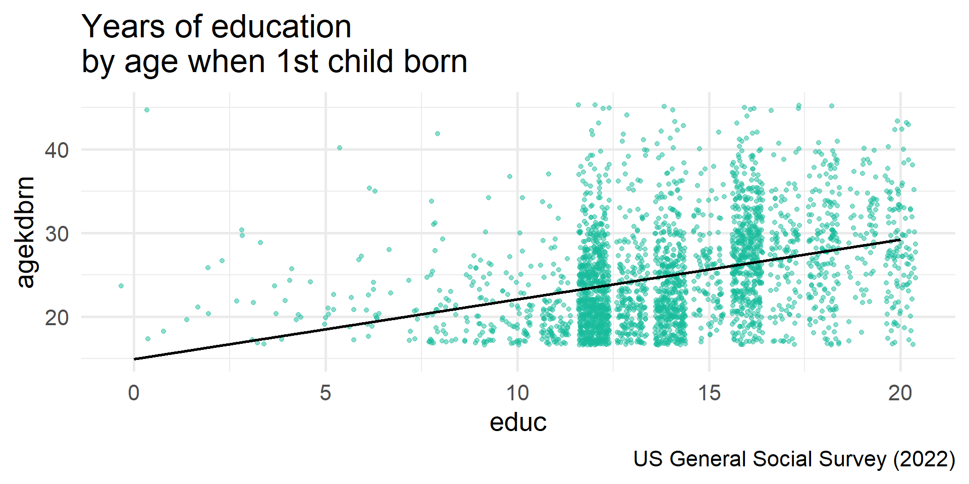
cor.test() in action

cor.test(
  ~ educ + agekdbrn,
  data = my_data,
  method = "pearson",
  na.action = na.omit
)

    Pearson's product-moment correlation

data:  educ and agekdbrn
t = 19.88, df = 2780, p-value < 2.2e-16
alternative hypothesis: true correlation is not equal to 0
95 percent confidence interval:
 0.3198258 0.3849110
sample estimates:
      cor 
0.3527951 

Tidy cor.test()

# Save results
my_test <- cor.test(
  ~ educ + agekdbrn,
  data = my_data,
  method = "pearson",
  na.action = na.omit
)

# Create a tibble with key stats
cor_summary <- tibble(
  correlation = my_test$estimate,
  p_value     = my_test$p.value,
  conf_low    = my_test$conf.int[1],
  conf_high   = my_test$conf.int[2]
)

cor_summary

# A tibble: 1 × 4
  correlation  p_value conf_low conf_high
        <dbl>    <dbl>    <dbl>     <dbl>
1       0.353 2.47e-82    0.320     0.385

cor.test() & t.test()

• Equivalence
• cor.test()
• t.test()

Heads Up!

Correlating a dichotomous variable and a continuous variable is equivalent to doing a t-test on that continuous variable by the dichotomous variable.

When x is coded as 0/1, these formulas yield equivalent p-values, even if the t-statistics look slightly different due to rounding or variance assumptions.

# Create numeric version of sex
my_data <- my_data %>%
  mutate(female = if_else(sex == "female", 1, 0))

cor.test(
  ~ female + lifenow,
  data = my_data,
  method = "pearson",
  na.action = na.omit
)

    Pearson's product-moment correlation

data:  female and lifenow
t = -0.85827, df = 2142, p-value = 0.3908
alternative hypothesis: true correlation is not equal to 0
95 percent confidence interval:
 -0.06082662  0.02381053
sample estimates:
        cor 
-0.01854126 

t.test(my_data$lifenow ~ my_data$sex, alternative = "two.sided")

    Welch Two Sample t-test

data:  my_data$lifenow by my_data$sex
t = 0.85806, df = 2137, p-value = 0.391
alternative hypothesis: true difference in means between group male and group female is not equal to 0
95 percent confidence interval:
 -0.07835816  0.20027032
sample estimates:
  mean in group male mean in group female 
            7.817837             7.756881 

Feature	t-test	Chi-square test	Pearson’s Correlation (R)
Purpose	Compare means between groups	Test association between categories	Measure linear relationship strength
Data Type	Continuous (numeric)	Categorical (nominal or ordinal)	Continuous (numeric)
Variables Required	1 dependent, 1 independent	2 categorical variables	2 continuous variables
Directionality	One-tailed or two-tailed	Non-directional	Indicates direction (+/-) and strength
Example Question	Do men and women differ in time spent on housework ?	Is marital status associated with political party identity?	Is there a correlation between number of children and parental stress?

Think Like a Statistician

Think Like a Statistician

Are beliefs about premarital sex (premarsx) dependent on political identity (polviews)?

Is there a gender difference (sex) in political identity (polviews)?

Describe the relationship between ageand life satisfaction (lifenow).

Think Like a Statistician

• premarsx
• polviews
• lifenow

Table 3

	polviews							Total
	extremely liberal	liberal	slightly liberal	moderate, middle of the road	slightly conservative	conservative	extremely conservative
premarsx
always wrong	7 (4.4%)	19 (5.1%)	16 (5.2%)	122 (12%)	48 (15%)	103 (28%)	44 (38%)	359 (14%)
almost always wrong	6 (3.8%)	11 (2.9%)	11 (3.6%)	55 (5.6%)	24 (7.3%)	36 (9.9%)	11 (9.5%)	154 (5.8%)
wrong only sometimes	7 (4.4%)	32 (8.6%)	33 (11%)	150 (15%)	59 (18%)	57 (16%)	13 (11%)	351 (13%)
not wrong at all	139 (87%)	311 (83%)	249 (81%)	657 (67%)	200 (60%)	169 (46%)	48 (41%)	1,773 (67%)
Total	159 (100%)	373 (100%)	309 (100%)	984 (100%)	331 (100%)	365 (100%)	116 (100%)	2,637 (100%)
Pearson’s Chi-squared test, p<0.001

Table 4

	sex		Total
	male	female
polviews
extremely liberal	103 (5.5%)	129 (6.0%)	232 (5.8%)
liberal	215 (12%)	347 (16%)	562 (14%)
slightly liberal	229 (12%)	247 (12%)	476 (12%)
moderate, middle of the road	661 (36%)	848 (40%)	1,509 (38%)
slightly conservative	267 (14%)	223 (10%)	490 (12%)
conservative	298 (16%)	258 (12%)	556 (14%)
extremely conservative	83 (4.5%)	92 (4.3%)	175 (4.4%)
Total	1,856 (100%)	2,144 (100%)	4,000 (100%)
Pearson’s Chi-squared test, p<0.001

    Pearson's product-moment correlation

data:  lifenow and age
t = 7.9037, df = 2031, p-value = 4.402e-15
alternative hypothesis: true correlation is not equal to 0
95 percent confidence interval:
 0.1302456 0.2146032
sample estimates:
      cor 
0.1727412