Statistical Tests I

Agenda

• Confidence Intervals
• Hypothesis Testing

• missing data?
• outliers
• dates?
• lists
• forcats (reorder factor levels)

Learning objectives

By the end of the lecture, you will be able to …

• Use R to calculate confidence intervals for means and proportions
• Use R to conduct one and two sample t-tests

Code-along 05

Download and open code-along-05.qmd

Mini-task

Install the Rmisc() package, available on CRAN.

Run the code chunk in your code-along.

OR: Copy and paste the code into your Console pane. Then hit “Enter”.

install.packages("Rmisc")

What does this mean in your code-along: “This chunk will not run (on purpose!) when rendered because eval: false.”?

We’ll use Rmisc() to calculate confidence intervals with summarize().

Mini-task

Load the standard packages and our new Rmisc() package.

library(tidyverse)
library(haven) # not core tidyverse
library(gssr)
library(gssrdoc) # load the GSS codebook
library(summarytools)
library(Rmisc) # load the new package

haven() was installed with tidyverse; but it doesn’t load automatically

Mini-task

Load the 2022 GSS data.

# Get the data from the 2022 survey
gss22 <- gss_get_yr(2022)

Variables

• wwwhr Not counting e-mail, about how many minutes or hours per week do you use the Web?
  
• postlife Do you believe there is a life after death?
  
• childs How many children have you ever had?
• sex Respondent’s sex

Mini-task

Create a dataset named my_data with the variables wwwhr, postlife, childs, & sex with no missing data

# Create a new df
my_data <-gss22 |>
  select(wwwhr, postlife, childs, sex) |>
  drop_na()

Confidence Intervals

Review: summarise()

my_data |>
  summarise(
    n = n(),
    mean = mean(wwwhr),
    sd = sd(wwwhr)
    )

# A tibble: 1 × 3
      n  mean    sd
  <int> <dbl> <dbl>
1   970  17.7  22.3

• CI
• SE

summarise() with equation

wwwhr_sum <- my_data |>
  summarise(
    n = n(),
    mean_wwwhr = mean(wwwhr),
    sd_wwwhr = sd(wwwhr),
    se_wwwhr = sd_wwwhr / sqrt(n),
    ci_lower = mean_wwwhr - (1.96 * se_wwwhr),
    ci_upper = mean_wwwhr + (1.96 * se_wwwhr)
    )

Code Meets Question

What can we infer about the population mean based on this confidence interval?

wwwhr_sum

# A tibble: 1 × 6
      n mean_wwwhr sd_wwwhr se_wwwhr ci_lower ci_upper
  <int>      <dbl>    <dbl>    <dbl>    <dbl>    <dbl>
1   970       17.7     22.3    0.716     16.3     19.1

summarise() + CI()

wwwhr_ci <- my_data |>
  summarise(
    n = n(),
    mean_wwwhr = mean(wwwhr),
    sd_wwwhr = sd(wwwhr),
    lowCI_wwwhr = Rmisc::CI(wwwhr)['lower'],
    hiCI_wwwhr  = Rmisc::CI(wwwhr)['upper']
    )

wwwhr_ci

# A tibble: 1 × 5
      n mean_wwwhr sd_wwwhr lowCI_wwwhr hiCI_wwwhr
  <int>      <dbl>    <dbl>       <dbl>      <dbl>
1   970       17.7     22.3        16.3       19.1

Neat! But how confident are we?

That’s really interesting, but don’t we need to know our confidence level? Otherwise, how do we interpret the interval? What is the probability that the average number of hours people spend on the internet per week is between 14.17 hours and 15.62 hours?

summarise() + CI()

wwwhr_ci99 <- my_data |>
  summarise(
    n = n(),
    mean_wwwhr = mean(wwwhr),
    sd_wwwhr = sd(wwwhr),
    lowCI_wwwhr = CI(wwwhr, ci = 0.99)['lower'],
    hiCI_wwwhr  = CI(wwwhr, ci = 0.99)['upper']
    )

wwwhr_ci99

# A tibble: 1 × 5
      n mean_wwwhr sd_wwwhr lowCI_wwwhr hiCI_wwwhr
  <int>      <dbl>    <dbl>       <dbl>      <dbl>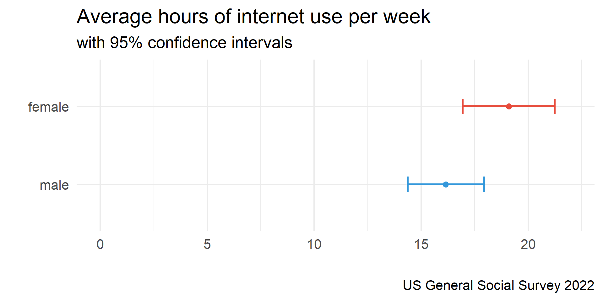
1   970       17.7     22.3        15.8       19.5

The default confidence level of the CI() function is 95%. Let’s change our code to see what the confidence interval looks like if we wanted to be 99% confident that the true population average number of hours on the internet was within our confidence interval.

CIs & percision

95% confidence intervals

wwwhr_ci

# A tibble: 1 × 5
      n mean_wwwhr sd_wwwhr lowCI_wwwhr hiCI_wwwhr
  <int>      <dbl>    <dbl>       <dbl>      <dbl>
1   970       17.7     22.3        16.3       19.1

99% confidence intervals

wwwhr_ci99

# A tibble: 1 × 5
      n mean_wwwhr sd_wwwhr lowCI_wwwhr hiCI_wwwhr
  <int>      <dbl>    <dbl>       <dbl>      <dbl>
1   970       17.7     22.3        15.8       19.5

How does a 95% confidence interval differ from a 99% confidence interval in terms of width and certainty?

CIs (wrong) with proportions

my_data |>
  summarise(
    n = n(),
    mean_ghosts = mean(postlife),
    sd_ghosts = sd(postlife),
    lowCI_ghosts = CI(postlife, ci = 0.99)['lower'],
    hiCI_ghosts  = CI(postlife, ci = 0.99)['upper']
    )

# A tibble: 1 × 5
      n mean_ghosts sd_ghosts lowCI_ghosts hiCI_ghosts
  <int>       <dbl>     <dbl>        <dbl>       <dbl>
1   970        1.19     0.389         1.15        1.22

This doesn’t work because the values aren’t coded 0 and 1.

CIs (correct) with proportions

# Use logic to recode (yes: 1 = 1; no: 2 = 0)
my_data$ghosts <- ifelse(my_data$postlife == 1, 1, 0)
  
my_data |>
  summarise(
    n = n(),
    mean_ghosts = mean(ghosts),
    sd_ghosts = sd(ghosts),
    lowCI_ghosts = CI(ghosts, ci = 0.99)['lower'],
    hiCI_ghosts  = CI(ghosts, ci = 0.99)['upper']
    )

# A tibble: 1 × 5
      n mean_ghosts sd_ghosts lowCI_ghosts hiCI_ghosts
  <int>       <dbl>     <dbl>        <dbl>       <dbl>
1   970       0.814     0.389        0.782       0.847

Comparing CIs

• Code
• Table
• Plot

my_data$sex <- zap_missing(my_data$sex) 
my_data$sex <- as_factor(my_data$sex)   
my_data$sex <- droplevels(my_data$sex)  

df_ghosts <- my_data |>
  group_by(sex) |>
  summarise(
    n = n(),
    mean = mean(ghosts),
    sd = sd(ghosts),
    lower = CI(ghosts, ci = 0.95)['lower'],
    upper  = CI(ghosts, ci = 0.95)['upper']
    )

df_ghosts

# A tibble: 2 × 6
  sex        n  mean    sd lower upper
  <fct>  <int> <dbl> <dbl> <dbl> <dbl>
1 male     472 0.773 0.419 0.735 0.811
2 female   498 0.853 0.354 0.822 0.885

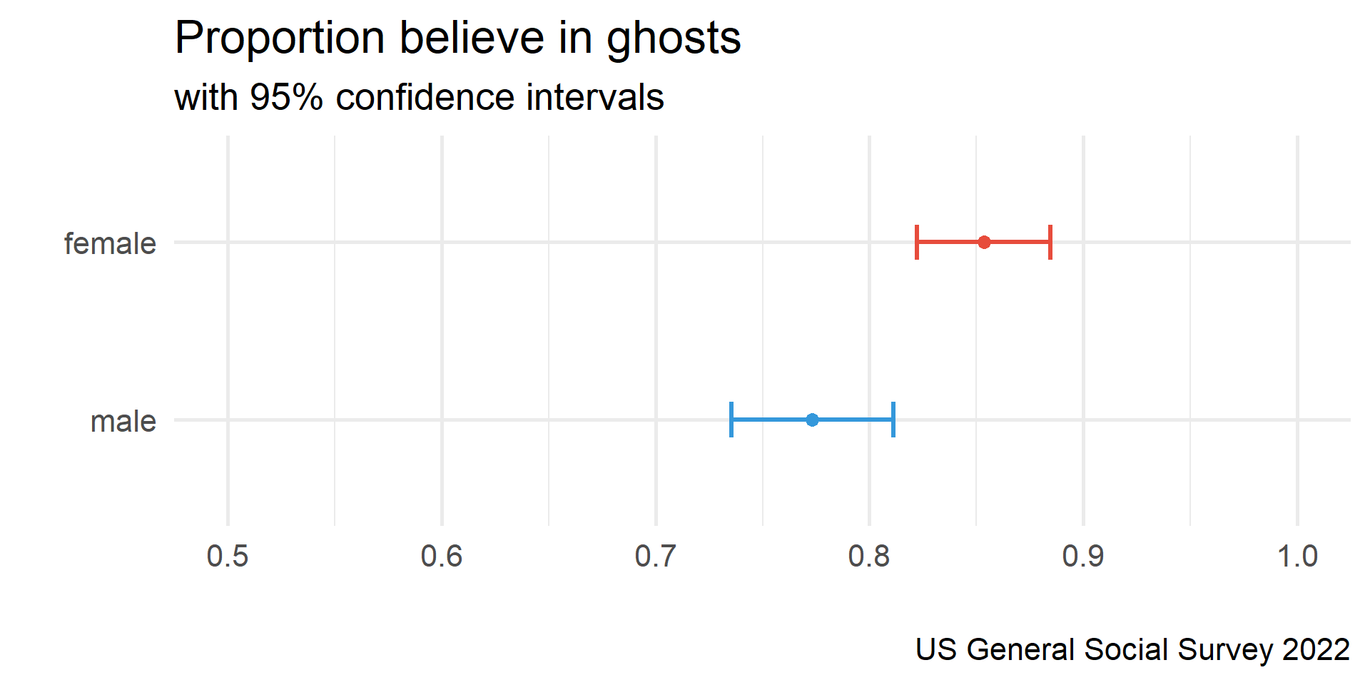
Comparing CIs

• Code
• Table
• Plot

df_wwwhr <- my_data |>
  group_by(sex) |>
  summarise(
    n = n(),
    mean = mean(wwwhr),
    sd = sd(wwwhr),
    lower = CI(wwwhr, ci = 0.95)['lower'],
    upper  = CI(wwwhr, ci = 0.95)['upper']
    )

df_wwwhr

# A tibble: 2 × 6
  sex        n  mean    sd lower upper
  <fct>  <int> <dbl> <dbl> <dbl> <dbl>
1 male     472  16.2  19.8  14.4  17.9
2 female   498  19.1  24.4  16.9  21.2

Hypothesis Testing

t.test()

Performs one and two sample t-tests. To use this function, we’ll need to specify a few things:

• variable of interest
• mu (H0): a number indicating the true value of the mean
• alternative hypothesis (H1): “two.sided”, “greater”, or “less”

t.test() in action

In your family sociology course you learned that fertility rates have been dropping.

You used to think that people had 2 children, on average. But, now you suspect that people are having fewer than 2 children.

How do you test your hypothesis?

Which of these equations represents your research hypothesis?

• H1: µ ≠ 2
• H1: µ = 2
• H1: µ < 2
• H1: µ > 2

Which of these equations represents your null hypothesis?

• H0: µ ≠ 2
• H0: µ = 2
• H0: µ < 2
• H0: µ > 2

Review: Summary Statistics

my_data |>
  summarise(
    n = n(),
    mean = mean(childs),
    median = median(childs),
    sd = sd(childs))

# A tibble: 1 × 4
      n  mean median    sd
  <int> <dbl>  <dbl> <dbl>
1   970  1.79      2  1.64

Is the difference between our sample mean and 2 statistically significant or could we have gotten this mean simply by chance (sample variation)?

Review: CIs

my_data |>
  summarise(
    n = n(),
    mean = mean(childs),
    median = median(childs),
    sd = sd(childs),
    se = sd / sqrt(n),
    lower = CI(childs, ci = 0.99)['lower'],
    upper  = CI(childs, ci = 0.99)['upper']
    )

# A tibble: 1 × 7
      n  mean median    sd     se lower upper
  <int> <dbl>  <dbl> <dbl>  <dbl> <dbl> <dbl>
1   970  1.79      2  1.64 0.0526  1.66  1.93

Does the confidence interval overlap with 2? What does that tell you?

One sample t.test() for means

t.test(my_data$childs)

    One Sample t-test

data:  my_data$childs
t = 34.102, df = 969, p-value < 2.2e-16
alternative hypothesis: true mean is not equal to 0
95 percent confidence interval:
 1.690587 1.897041
sample estimates:
mean of x 
 1.793814 

H0 = 0 by default

One sample t.test() for means

t.test(my_data$childs, mu=2, alternative="less") # Ho: mu=2

    One Sample t-test

data:  my_data$childs
t = -3.9197, df = 969, p-value = 4.744e-05
alternative hypothesis: true mean is less than 2
95 percent confidence interval:
    -Inf 1.88042
sample estimates:
mean of x 
 1.793814 

H0 = 2; one-tail test

Assuming an α level of .05, should you reject the null hypothesis?

• No, because the 𝛼 level of .01 is greater than the p-value (< .000).
• No, because the p-value (< .000) is less than the 𝛼 level of .01.
• Yes, because the p-value (< .000) is less than the 𝛼 level of .01.

Which of these statements best summarizes your conclusion?

• Our evidence proves that people have fewer than two children, on average.
• People, on average, have two children.
• On average, the number of children people have is statistically significantly lower than two.

two sample t.test() in action

Are the proportions of men and women who believe in ghosts statistically significantly different?

t.test(my_data$ghosts ~ my_data$sex, alternative = "two.sided")

    Welch Two Sample t-test

data:  my_data$ghosts by my_data$sex
t = -3.2072, df = 923.29, p-value = 0.001387
alternative hypothesis: true difference in means between group male and group female is not equal to 0
95 percent confidence interval:
 -0.1291289 -0.0310882
sample estimates:
  mean in group male mean in group female 
           0.7733051            0.8534137 

Assuming an α level of .05, what do you conclude?

• There is no statistically significant difference between men and women in belief in ghosts.
• Men are significantly more likely than women to believe in ghosts (p < .05).
• Women are significantly more likely than men to believe in ghosts (p < .05).

Aside: paired t.test()

Independent group t-test
Do two subsamples have the same mean?

t.test(my_data$ghosts ~ my_data$sex, alternative = "two.sided")

Paired t-test
Do two variables have the same mean?

t.test(Pair(hrs1_2018, hrs1_2020) ~ 1, data = gss_panel)

Think Like a Statistician

Think Like a Statistician

Do women have more years of education (educ) than men, on average?

Are the proportions of men & women who support abortion for any reason (abany) statistically different?

Do fewer men than women support gun laws (gunlaw)?

Use the 2022 GSS dataset

Think Like a Statistician

• educ
• abany
• gunlaw

    Welch Two Sample t-test

data:  gss22$educ by gss22$sex
t = -0.38076, df = 4035.7, p-value = 0.3517
alternative hypothesis: true difference in means between group 1 and group 2 is less than 0
95 percent confidence interval:
      -Inf 0.1144853
sample estimates:
mean in group 1 mean in group 2 
       14.14338        14.17786 

    Welch Two Sample t-test

data:  gss22$abany by gss22$sex
t = -1.0701, df = 1317.7, p-value = 0.2848
alternative hypothesis: true difference in means between group 1 and group 2 is not equal to 0
95 percent confidence interval:
 -0.08169512  0.02402811
sample estimates:
mean in group 1 mean in group 2 
      0.5786164       0.6074499 

    Welch Two Sample t-test

data:  gss22$gunlaw by gss22$sex
t = -8.9698, df = 2476.6, p-value < 2.2e-16
alternative hypothesis: true difference in means between group 1 and group 2 is not equal to 0
95 percent confidence interval:
 -0.1872801 -0.1200856
sample estimates:
mean in group 1 mean in group 2 
      0.6450593       0.7987421