Introduction to Data

Agenda

• Coding Basics
• Variable Types
• Frequency Distributions

What questions do we have from the tutorial??

Learning objectives

By the end of the lecture, you will be able to …

• use R to conduct basic calculations/comparisons
• identify and convert variable types
• create useful frequency tables

Code-along 02

Download code-along-02.qmd

Mini-task

Install the summarytools() package, available on CRAN.

Run the code chunk in your code-along.

OR: Copy and paste the code into your Console pane. Then hit “Enter”.

install.packages("summarytools")

What does this mean in your code-along: “This chunk will not run (on purpose!) when rendered because eval: false.”?

Mini-task

Load the standard packages and our new summarytools() package.

library(tidyverse)
library(haven) # not core tidyverse
library(gssr)
library(gssrdoc) # load the GSS codebook
library(summarytools)

haven() was installed with tidyverse; but it doesn’t load automatically

Mini-task

Load the 2024 GSS data.

# Get the data only for the 2024 survey respondents
gss24 <- gss_get_yr(2024)

Why did we need to use library() before we loaded the GSS data?

Coding Basics

Coding basics

You can use R to do basic math calculations

1 + 2

[1] 3

2 * 5

[1] 10

(1 + 2) / 2

[1] 1.5

You can create new objects with the assignment operator <-

x <- 3 * 4
x

[1] 12

You can (and should) make comments in your code

# R will ignore any text after # for that line

primes <- c(2, 3, 5, 7, 11, 13) # create vector of prime numbers
primes

[1]  2  3  5  7 11 13

Object names must start with a letter and can only contain letters, numbers, _, and .

i_use_snake_case
otherPeopleUseCamelCase
some.people.use.periods
And_aFew.People_RENOUNCEconvention

Source: R for Data Science

Coding basics: demo

a <- 7
b <- 3
addition <- a + b
subtraction <- a - b
multiplication <- a * b
division <- a / b
exponentiation <- a^2

a

[1] 7

b

[1] 3

addition

[1] 10

subtraction

[1] 4

multiplication

[1] 21

division

[1] 2.333333

exponentiation

[1] 49

Operators in R

Operators in R are symbols directing R to perform various kinds of mathematical, logical, and decision operations. A few of the key ones to know before we get started:

Assignment operators assign values to variables:
<-, ->, =

Comparison operators test equality or inequality:
==, !=, >, >=, <, <=

Logical operators indicate “and”, “or”, and “not”:
&, |, !

Comparison operators

operator	definition
<	is less than?
<=	is less than or equal to?
>	is greater than?
>=	is greater than or equal to?
==	is exactly equal to?
!=	is not equal to?

Comparison operators (cont)

x <- 5
y <- 3
equal <- x == y
not_equal <- x != y
less_than <- x < y
more_than <- x > y
less_than_or_equal_to <- x <= y
more_than_or_equal_to <- x >= y

x

[1] 5

y

[1] 3

equal

[1] FALSE

not_equal

[1] TRUE

less_than

[1] FALSE

more_than

[1] TRUE

less_than_or_equal_to

[1] FALSE

more_than_or_equal_to

[1] TRUE

Source: IONOS editorial team

Logical operators

operator	definition
x & y	is x AND y?
x | y	is x OR y?
is.na(x)	is x NA?
!is.na(x)	is x not NA?

Logical operators (cont)

x <- TRUE
y <- FALSE

and_operator <- x & y
or_operator <- x | y
not_operator <- !x

and_operator

[1] FALSE

or_operator

[1] TRUE

not_operator

[1] FALSE

Source: IONOS editorial team

Mini-task

Make a tiny data frame and save it.

df <- tibble(x = c(1, 2, 3, 4, 5), y = c("a", "a", "b", "c", "c"))

df # look at df

# A tibble: 5 × 2
      x y    
  <dbl> <chr>
1     1 a    
2     2 a    
3     3 b    
4     4 c    
5     5 c    

Variable Types

Data types in R

A property is assigned to objects that determines how generic functions operate with it.

Common ‘types’ or ‘classes’ of variables:

• logical
• character
• integer
• numeric
• and more, but we won’t be focusing on those

Data class + variable type

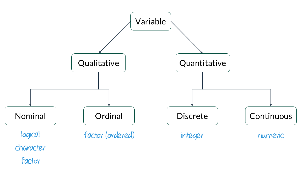
class()

logical - Boolean values TRUE and FALSE

class(TRUE)

[1] "logical"

character - character strings

class("Sociology")

[1] "character"

Integer - numeric data without decimals
(indicated with an L).

class(2L)

[1] "integer"

numeric - default type if values are numbers or if the values contain decimals.

class(2.5)

[1] "numeric"

Factor

factors consist of character data with a fixed and known set of possible values

opinion <- factor(c("like", "dislike", "dislike", "hate", "dislike", "hate"))
class(opinion)

[1] "factor"

# By default, the levels are sorted alphabetically.
levels(opinion)

[1] "dislike" "hate"    "like"   

Factor order

# Reorder the levels with the argument `levels` in the `factor()` function
opinion <- factor(opinion, levels = c("hate", "dislike", "like"))
levels(opinion)

[1] "hate"    "dislike" "like"   

# If the order has meaning (like rankings), you can make it an ordered factor
opinion <- factor(opinion, levels = c("hate", "dislike", "like"), ordered = TRUE)
levels(opinion)

[1] "hate"    "dislike" "like"   

Converting between types

Use a function: as.logical(), as.numeric(), as.integer(), or as.character().

Create a numeric variable.

x <- 1:3
x

[1] 1 2 3

class(x)

[1] "integer"

Heads Up!

The : (colon) means ‘through.’

Change it to a character variable.

y <- as.character(x)
y

[1] "1" "2" "3"

class(y)

[1] "character"

Heads Up!

Notice the quotation marks around the values.

Haven labelled

When you import data into R from software like SPSS, Stata, or SAS, you might notice a special class called haven_labelled.

class(gss24$premarsx)

[1] "haven_labelled" "vctrs_vctr"     "double"        

table(gss24$premarsx)

   1    2    3    4 
 357  122  258 1378 

Haven labelled cont.

It makes data easier to understand without needing a separate codebook.

attr(gss24$premarsx, "label")
print_labels(gss24$premarsx)

1

A description of the variable

2

View the label attached to each numeric value

[1] "sex before marriage"

Labels:
 value                         label
     1                  always wrong
     2           almost always wrong
     3          wrong only sometimes
     4              not wrong at all
     5                         other
 NA(d)                    don't know
 NA(i)                           iap
 NA(j)            I don't have a job
 NA(m)                   dk, na, iap
 NA(n)                     no answer
 NA(p)                 not imputable
 NA(r)                       refused
 NA(s)                skipped on web
 NA(u)                    uncodeable
 NA(x) not available in this release
 NA(y)    not available in this year
 NA(z)                  see codebook

The column itself might have a variable label (a description like “Gender of respondent”)

The column contains values (numbers)

Each value may have a label attached (like “Male” for 1, “Female” for 2)

You can use as_factor to see the value labels of the variable premarsx.

• Mini-task
• with as_factor()
• without as_factor()

Use as_factor() inside the table() function for the variable premarsx

table(as_factor(gss24$premarsx), useNA = "ifany")

                 always wrong           almost always wrong 
                          357                           122 
         wrong only sometimes              not wrong at all 
                          258                          1378 
                        other                           iap 
                            0                          1126 
                   don't know            I don't have a job 
                           50                             0 
                  dk, na, iap                     no answer 
                            0                             6 
                not imputable                       refused 
                            0                             0 
               skipped on web                    uncodeable 
                           12                             0 
not available in this release    not available in this year 
                            0                             0 
                 see codebook 
                            0 

table(gss24$premarsx, useNA = "ifany")

   1    2    3    4 <NA> 
 357  122  258 1378 1194 

In the code-along, REPLACE THE BLANK LINE WITH THE NAME OF THE VARIABLE

What would happen if we didn’t include as_factor() within table()?

Convert labels to factors

• zap_missing()
• as_factor()
• droplevels()

1. Use zap_missing() to get rid of all the ‘missing’ (NA) levels

gss24$premarsx <- zap_missing(gss24$premarsx)
table(as_factor(gss24$premarsx), useNA = "ifany") # see the results

        always wrong  almost always wrong wrong only sometimes 
                 357                  122                  258 
    not wrong at all                other                 <NA> 
                1378                    0                 1194 

2. Use as_factor() to apply the labels instead of numeric values

gss24$premarsx <- as_factor(gss24$premarsx) # replace the values with labels
table(gss24$premarsx, useNA = "ifany") # notice we didn't need to wrap the variable in as_factor

        always wrong  almost always wrong wrong only sometimes 
                 357                  122                  258 
    not wrong at all                other                 <NA> 
                1378                    0                 1194 

3. Use droplevels() to get rid of the empty levels in premarsx.

gss24$premarsx <- droplevels(gss24$premarsx)
table(gss24$premarsx)

        always wrong  almost always wrong wrong only sometimes 
                 357                  122                  258 
    not wrong at all 
                1378 

1. REPLACE THE BLANK LINES WITH THE NAME OF THE VARIABLE
   
2. REPLACE THE BLANK LINE WITH THE FUNCTION as_factor()
   
3. REPLACE THE BLANK LINES WITH THE droplevels() function & the NAME OF THE VARIABLE

Mini-task

Use zap_missing(), as_factor(), & droplevels() on the variable sex.

gss24$sex <- zap_missing(gss24$sex)
gss24$sex <- as_factor(gss24$sex)
gss24$sex <- droplevels(gss24$sex)

table(gss24$sex)

1

Get rid of all the ‘missing’ (NA) levels.

2

Replace the values with labels.

3

Get rid of the empty levels (if any).

  male female 
  1467   1823 

use zap_missing(), as_factor(), and droplevels() to do the same for the sex variable.

Frequency Distributions

Relative frequency table

Let’s try functions from the summarytools() package to get univariate (1 variable) and bivariate (2 variables) descriptive statistics.

freq() creates table of the counts for a variable.

freq(gss24$sex)

Frequencies  
gss24$sex  
Type: Factor  

               Freq   % Valid   % Valid Cum.   % Total   % Total Cum.
------------ ------ --------- -------------- --------- --------------
        male   1467     44.59          44.59     44.33          44.33
      female   1823     55.41         100.00     55.09          99.43
        <NA>     19                               0.57         100.00
       Total   3309    100.00         100.00    100.00         100.00

To use the freq() function, what did we need to do first? AK: Load the summarytools() package.

Mini-task

Use freq() on the variable premarsx

freq(gss24$premarsx)

Frequencies  
gss24$premarsx  
Type: Factor  

                             Freq   % Valid   % Valid Cum.   % Total   % Total Cum.
-------------------------- ------ --------- -------------- --------- --------------
              always wrong    357     16.88          16.88     10.79          10.79
       almost always wrong    122      5.77          22.65      3.69          14.48
      wrong only sometimes    258     12.20          34.85      7.80          22.27
          not wrong at all   1378     65.15         100.00     41.64          63.92
                      <NA>   1194                              36.08         100.00
                     Total   3309    100.00         100.00    100.00         100.00

Pretty tables

One of summarytools main purposes is to help clean and prepare data for further analysis. But sometimes we don’t care about the missing values.

Using report.nas = FALSE suppresses the missing data.
The headings = FALSE parameter suppresses the heading section.

freq(gss24$sex, report.nas = FALSE, headings = FALSE)

               Freq        %   % Cum.
------------ ------ -------- --------
        male   1467    44.59    44.59
      female   1823    55.41   100.00
       Total   3290   100.00   100.00

Mini-task

Make a pretty frequency table for the variable premarsx.

freq(gss24$premarsx, report.nas = FALSE, headings = FALSE)

                             Freq        %   % Cum.
-------------------------- ------ -------- --------
              always wrong    357    16.88    16.88
       almost always wrong    122     5.77    22.65
      wrong only sometimes    258    12.20    34.85
          not wrong at all   1378    65.15   100.00
                     Total   2115   100.00   100.00

Cross-tabs

We’ve been using the table() function with one variable at a time, but it also let’s you create a frequency table (crosstab) with two variables.

# 1st variable is the rows, 2nd variable is the columns.
table(gss24$premarsx, gss24$sex)

                      
                       male female
  always wrong          146    209
  almost always wrong    44     77
  wrong only sometimes  127    130
  not wrong at all      616    758

But it’s missing the column percentages…

Relative frequency by group

To run freq() by group, pair it with the stby() function.

stby(gss24$premarsx, gss24$sex, freq)

Frequencies  
gss24$premarsx  
Type: Factor  
Group: sex = male  

                             Freq   % Valid   % Valid Cum.   % Total   % Total Cum.
-------------------------- ------ --------- -------------- --------- --------------
              always wrong    146     15.65          15.65      9.95           9.95
       almost always wrong     44      4.72          20.36      3.00          12.95
      wrong only sometimes    127     13.61          33.98      8.66          21.61
          not wrong at all    616     66.02         100.00     41.99          63.60
                      <NA>    534                              36.40         100.00
                     Total   1467    100.00         100.00    100.00         100.00

Group: sex = female  

                             Freq   % Valid   % Valid Cum.   % Total   % Total Cum.
-------------------------- ------ --------- -------------- --------- --------------
              always wrong    209     17.80          17.80     11.46          11.46
       almost always wrong     77      6.56          24.36      4.22          15.69
      wrong only sometimes    130     11.07          35.43      7.13          22.82
          not wrong at all    758     64.57         100.00     41.58          64.40
                      <NA>    649                              35.60         100.00
                     Total   1823    100.00         100.00    100.00         100.00

This is hard to read and we don’t need the cumulative frequencies.

stby() lets us obtain grouped statistics with summarytools functions

Pretty cross-tabs with ctable()

Use summarytools::ctable instead!

ctable(gss24$premarsx, gss24$sex,
  prop = "c",
  format = "p",
  useNA = "no"
)

1

Change from table() to ctable().

2

The “c” gives column %; “r” would give row %.

3

This adds the % symbols to the table.

4

Exclude the missing levels from the table.

Cross-Tabulation, Column Proportions  
premarsx * sex  
Data Frame: gss24  

---------------------- ----- -------------- --------------- ---------------
                         sex           male          female           Total
              premarsx                                                     
          always wrong         146 ( 15.6%)    209 ( 17.8%)    355 ( 16.8%)
   almost always wrong          44 (  4.7%)     77 (  6.6%)    121 (  5.7%)
  wrong only sometimes         127 ( 13.6%)    130 ( 11.1%)    257 ( 12.2%)
      not wrong at all         616 ( 66.0%)    758 ( 64.6%)   1374 ( 65.2%)
                 Total         933 (100.0%)   1174 (100.0%)   2107 (100.0%)
---------------------- ----- -------------- --------------- ---------------

Add to your code-along: 1. X percentage of respondents believe sex before marriage is ‘almost always wrong’?
2. A greater percentage of X think sex before marriage is ‘not wrong at all’.

Based on your table, what percentage of respondents believe sex before marriage is ‘almost always wrong’?

• 5.7
• 16.8
• 121
• 12.2

Based on your table, do a greater percentage of men or women think sex before marriage is ‘not wrong at all’?

• Men
• Women