R workflow

Agenda

• R & RStudio Workflow
• Quarto
• Getting Started

Learning objectives

By the end of the lecture, you will be able to …

• setup a workflow using R and RStudio
  
• familiarize yourself with a dataset using R and RStudio
  
• create a reproducible report using Quarto
  

R & RStudio Tour

Tour: RStudio Panes

Sit back and enjoy the show!

• open new R script
  
• Environment (data values, functions)
• Plots, Help, Viewer
• Console – typing

Mini-task

Open a new R Script.

Click the dropdown arrow next to the “New File icon,” and then “R script”.

An R-script is a file that will contain the documentation of the code of what you tell R to do.

Alternatively, hold down “Ctrl” + “Shift” + “N.”

Mini-tasks

Type 2 + 2 in the Console. Then push Enter.

Type 2 + 2 in the R Script Then click Run.

What’s the difference between the console and a script file?

Documentation

In .R scripts and Quarto, you can document your code. Err on the side of over documentation. Your future self will thank you. In .R scripts, the way to make a comment rather than a command, is to put a pound sign in front of the text.

Mini-task

Add a comment above your 2 + 2 code in your R script. Then click Run.

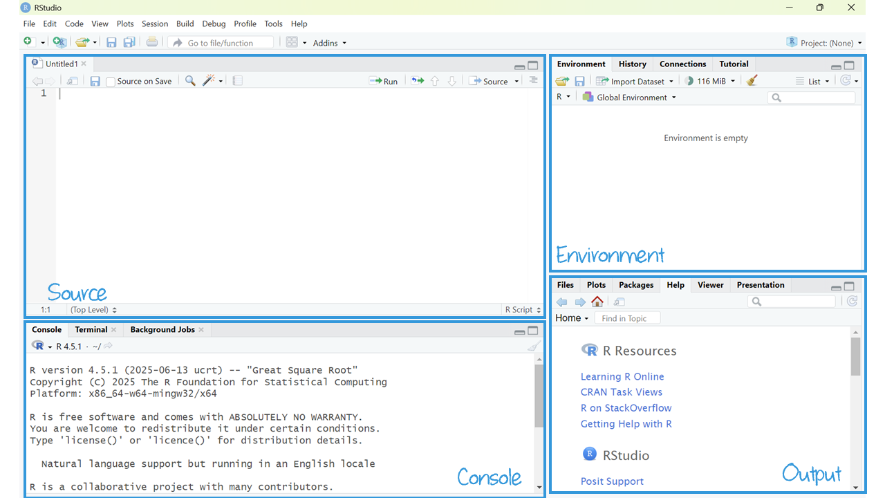
Tour recap: Panes

There are four key regions or “panes” in the interface:

1. Source pane: where you can edit and save R scripts or author computational documents like Quarto and R Markdown.

2. Console pane: is used to write short interactive R commands.

3. Environment pane: displays temporary R objects created during that R session.

4. Output pane: displays the plots, tables, or HTML outputs of executed code along with files saved to disk.

Heads Up!

The top-left panel (source pane) and can be launched by opening any editable file in RStudio.

Console pane: best for exploring.
Source pane: best for documenting.

RStudio projects

Create a RStudio project for each data analysis project.

It supports an organized and reproducible workflow, cleanly separated from all other projects that you are working on. Everything you need in one place:

• local data files to load into RStudio.
• scripts to edit or run in bits or as a whole.
• Save your outputs (plots and cleaned data).

Source: https://docs.posit.co/ide/user/ide/get-started/#hello-rstudio-projects

File types

There are many file types, but these are key to an R & RStudio workflow (and likely new to you):

Extension	Description
.Rproj	RStudio project file (keeps project settings).
.R	R scripts store a sequence of R commands (code) that can be run all at once or line by line.
.qmd	Quarto Markdown creates reproducible documents that contain a combination of text, code, and output.
.Rdata (or sometimes .rda)	These store and load R objects—like data frames.

Mini-task

Create a new project in RStudio.

• Click: File > New Project.

• In the New Project wizard that pops up, select: New Directory, then New Project.

• Name the project “SOC6302”

• Click Browse and save the project anywhere except your downloads folder.

• Click: Create Project.

• This will launch you into a new RStudio Project inside a new folder called “SOC6302”.

Mini-task

Clear the memory at every restart of RStudio.

Turn off theautomatic saving of your workspace and .Rdata files with you quit RStudio. This is important for reproducibility, debugging, and avoiding littering your computer with unnecessary files.

Set this via:

1. Tools > Global Options.
2. Uncheck “Restore .RData into Workspace at Startup”.
3. Choose “Never” on the “Save workspace to .RData on exit”.
4. Click “Apply” and “OK”.

Quarto

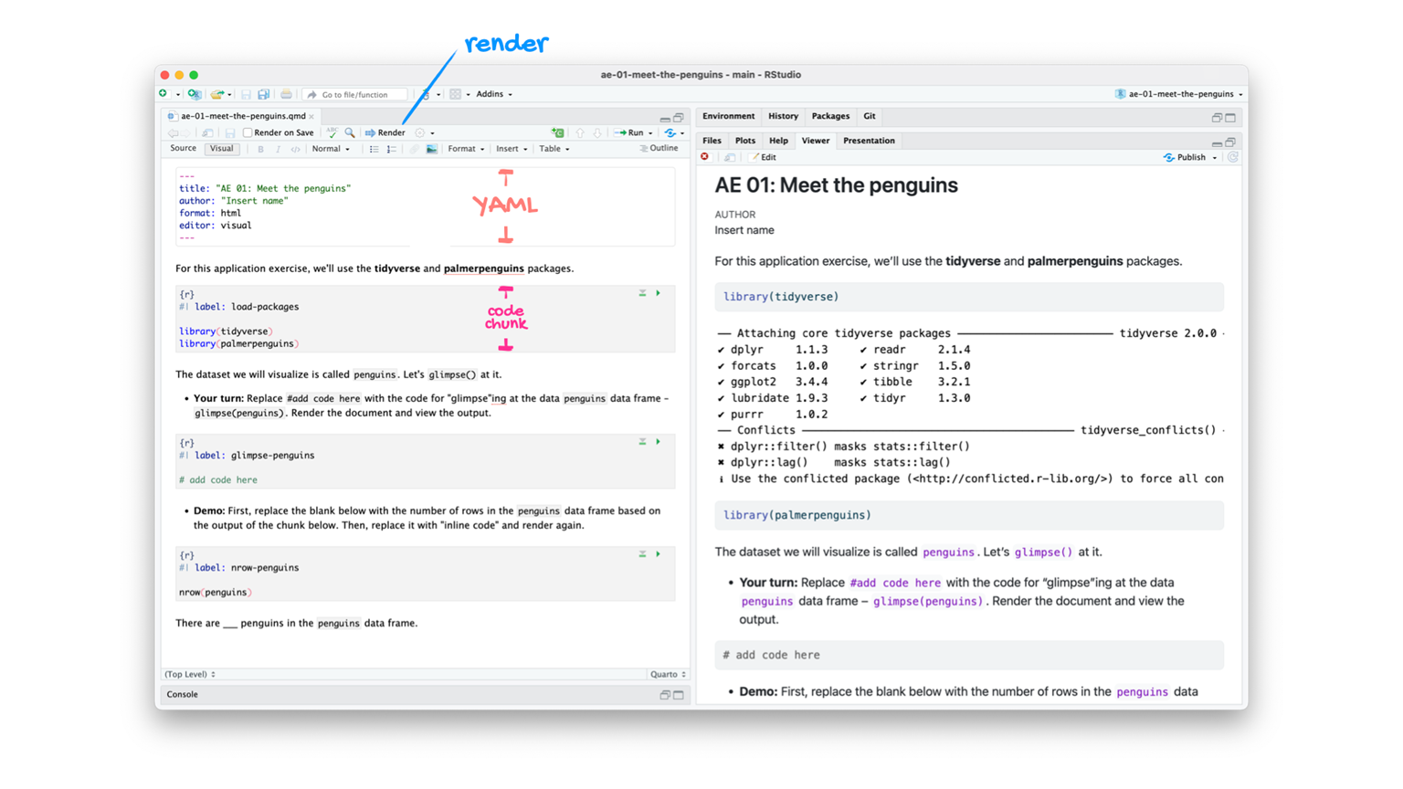
Quarto

The tool you’ll use to create reproducible computational documents. Every piece of assignment you hand in will be a Quarto document.

• Fully reproducible reports
• R code + narrative

You are likely familiar with word processors like MS Word or Google Docs. We will not be using these in this class. Instead, the words you would write in such a document, as well as your R code, will go into a Quarto document. You will render the document (more on what this means later) to get a document out that has your words, code, and the output of that code. Everything in one place, beautifully formatted!

RScript

• great for learning, exploring and tinkering.

• rerun it without attention to formatting or markdown.

Quarto

• great for communicating analysis and results

• combines narrative explanation with code output (results).

Tour: Quarto

Sit back and enjoy the show!

• open new Quarto doc as an example
• YAML Ain’t Markup Language
• code chunk (+ code comments)
• type 2 + 2 in Quarto chunk
• add narrative (no hashtags)
• code chunk options
• narrative (heading levels)
• run (line vs code chunk)
• run cells above
• source and visual
• render

Tour recap: Quarto

Source: Dr. Mine Çetinkaya-Rundel

Tour recap: Quarto Code-chunks

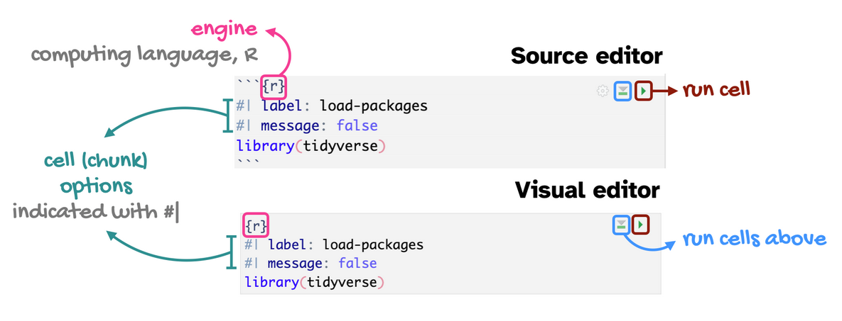
• chunk labels are helpful for describing what the code is doing, for jumping between code cells in the editor, and for troubleshooting
• message: false hides any messages emitted by the code in your rendered document

Source: Dr. Mine Çetinkaya-Rundel

How will we use Quarto?

• Every code-along and milestone will be a Quarto document
• The scaffolding will decrease over the course
• You will create and submit a Quarto document for your research project

Tutorial: Hello, Quarto

Your first code-along

Download code-along-01.qmd

Mini-task

Save this code-along in your newly created project folder.

There’s no command in the R console to save scripts or Quarto files— you use the editor’s File > Save As or Ctrl+S.

Getting Started

Comprehensive R Archive Network (CRAN)

CRAN is like an App Store for R. It hosts R packages, documentation, and source code contributed by users worldwide. It is mediated (e.g., quality controlled), making it incredibly reliable.

Packages

R comes with basic tools, but packages extend the capabilities of base R (what you already installed). An R package is like a toolbox: a collection of functions, data, and documentation that help you do specific tasks using R.

You’ll install each package (1X per system):

install.packages("tidyverse")

You’ll load each package (every time you use it):

library(tidyverse)

What’s the difference between installing and loading a package? Why is this annoying workflow a “feature”?

Mini-task

Install the tidyverse() package, available on CRAN.

Run the code chunk in your code-along.

OR: Copy and paste the code into your Console pane. Then hit “Enter”.

install.packages("tidyverse")

Mini-tasks

Install the tinytex() package, available on CRAN.

Run the code chunk in your code-along.

OR: Copy and paste the code into your Console pane. Then hit “Enter”.

install.packages('tinytex')

tinytex::install_tinytex()

Mini-tasks

Install the gssr() package, NOT on CRAN.

# Install 'gssr' from 'ropensci' universe
install.packages('gssr', repos =
  c('https://kjhealy.r-universe.dev', 'https://cloud.r-project.org'))

Install the gssrdoc() package, NOT on CRAN.

# Install 'gssrdoc' from 'ropensci' universe
install.packages('gssrdoc', repos =
  c('https://kjhealy.r-universe.dev', 'https://cloud.r-project.org'))

Mini-task

Load the packages.

Run the code chunk in your code-along.

library(tidyverse) # for data wrangling
library(gssr) # U.S. General Social Survey data
library(gssrdoc) # GSS documentation

Environment

Run the code chunk in your code-along.

# software documentation
sessionInfo()

R version 4.5.1 (2025-06-13 ucrt)
Platform: x86_64-w64-mingw32/x64
Running under: Windows 11 x64 (build 26100)

Matrix products: default
  LAPACK version 3.12.1

locale:
[1] LC_COLLATE=English_Canada.utf8  LC_CTYPE=English_Canada.utf8   
[3] LC_MONETARY=English_Canada.utf8 LC_NUMERIC=C                   
[5] LC_TIME=English_Canada.utf8    

time zone: America/Toronto
tzcode source: internal

attached base packages:
[1] stats     graphics  grDevices utils     datasets  methods   base     

other attached packages:
 [1] gssrdoc_0.7.0      conflicted_1.2.0   summarytools_1.1.4 flextable_0.9.7   
 [5] kableExtra_1.4.0   labelled_2.14.1    haven_2.5.5        gssr_0.7          
 [9] lubridate_1.9.4    forcats_1.0.0      stringr_1.5.1      dplyr_1.1.4       
[13] purrr_1.0.4        readr_2.1.5        tidyr_1.3.1        tibble_3.3.0      
[17] ggplot2_3.5.2      tidyverse_2.0.0   

loaded via a namespace (and not attached):
 [1] gtable_0.3.6            xfun_0.52               tzdb_0.5.0             
 [4] vctrs_0.6.5             tools_4.5.1             generics_0.1.4         
 [7] curl_6.3.0              pacman_0.5.1            pkgconfig_2.0.3        
[10] data.table_1.17.6       checkmate_2.3.2         pryr_0.1.6             
[13] RColorBrewer_1.1-3      uuid_1.2-1              lifecycle_1.0.4        
[16] compiler_4.5.1          farver_2.1.2            rapportools_1.2        
[19] textshaping_1.0.1       codetools_0.2-20        fontquiver_0.2.1       
[22] fontLiberation_0.1.0    htmltools_0.5.8.1       yaml_2.3.10            
[25] pillar_1.11.0           MASS_7.3-65             openssl_2.3.3          
[28] cachem_1.1.0            magick_2.8.7            fontBitstreamVera_0.1.1
[31] tidyselect_1.2.1        zip_2.3.3               digest_0.6.37          
[34] stringi_1.8.7           reshape2_1.4.4          pander_0.6.6           
[37] fastmap_1.2.0           grid_4.5.1              cli_3.6.5              
[40] magrittr_2.0.3          base64enc_0.1-3         withr_3.0.2            
[43] backports_1.5.0         gdtools_0.4.1           scales_1.4.0           
[46] timechange_0.3.0        rmarkdown_2.29          officer_0.6.7          
[49] matrixStats_1.5.0       askpass_1.2.1           ragg_1.4.0             
[52] hms_1.1.3               memoise_2.0.1           evaluate_1.0.4         
[55] knitr_1.50              tcltk_4.5.1             viridisLite_0.4.2      
[58] rlang_1.1.6             Rcpp_1.0.14             glue_1.8.0             
[61] xml2_1.3.8              svglite_2.1.3           rstudioapi_0.17.1      
[64] jsonlite_2.0.0          plyr_1.8.9              R6_2.6.1               
[67] systemfonts_1.2.3       fs_1.6.6               

Meet your data

We’re going to use data from the U.S. General Social Survey (GSS).

Who knows what the GSS is?

Load some data

Run the code chunk in your code-along.

# Load the data (will appear in your Global Environment pane)
gss24 <- gss_get_yr(2024)

# Preview the data named gss24
gss24

# A tibble: 3,309 × 813
   year       id wrkstat hrs1        hrs2        evwork      wrkslf  occ10      
   <dbl+l> <dbl> <dbl+l> <dbl+lbl>   <dbl+lbl>   <dbl+lbl>   <dbl+l> <dbl+lbl>  
 1 2024        1 1 [wor…    43       NA(i) [iap] NA(i) [iap] 2 [som…   230 [edu…
 2 2024        2 5 [ret… NA(i) [iap] NA(i) [iap]     1 [yes] 2 [som…   800 [acc…
 3 2024        3 5 [ret… NA(i) [iap] NA(i) [iap]     1 [yes] 2 [som…   430 [man…
 4 2024        4 2 [wor…    20       NA(i) [iap] NA(i) [iap] 2 [som…  4760 [ret…
 5 2024        5 5 [ret… NA(i) [iap] NA(i) [iap]     1 [yes] 2 [som…  5860 [off…
 6 2024        6 4 [une… NA(i) [iap] NA(i) [iap] NA(i) [iap] 1 [sel…  4000 [che…
 7 2024        7 1 [wor…    80       NA(i) [iap] NA(i) [iap] 2 [som…  9640 [pac…
 8 2024        8 6 [in … NA(i) [iap] NA(i) [iap]     1 [yes] 2 [som…  3600 [nur…
 9 2024        9 1 [wor…    50       NA(i) [iap] NA(i) [iap] 2 [som… NA(n) [no …
10 2024       10 4 [une… NA(i) [iap] NA(i) [iap] NA(i) [iap] 2 [som…  5620 [sto…
# ℹ 3,299 more rows
# ℹ 805 more variables: prestg10 <dbl+lbl>, prestg105plus <dbl+lbl>,
#   indus10 <dbl+lbl>, marital <dbl+lbl>, martype <dbl+lbl>, divorce <dbl+lbl>,
#   widowed <dbl+lbl>, spwrksta <dbl+lbl>, sphrs1 <dbl+lbl>, sphrs2 <dbl+lbl>,
#   spevwork <dbl+lbl>, cowrksta <dbl+lbl>, cowrkslf <dbl+lbl>,
#   coevwork <dbl+lbl>, cohrs1 <dbl+lbl>, cohrs2 <dbl+lbl>, spwrkslf <dbl+lbl>,
#   spocc10 <dbl+lbl>, sppres10 <dbl+lbl>, sppres105plus <dbl+lbl>, …

A “tibble” is another name for “tidy dataset,” meaning that the data is organized in structured, clear rows and columns. “(3309 × 639)” means the dataset contains 3309 rows and 639 columns. Commonly, in social sciences, rows are referred to as “observations” and columns as “variables.” In our case, there are 639 observations (e.g., respondents) and 639 variables.

Browse dataframe

Open the gss24 dataframe.

With your mouse, go to the environment panel (upper-right) and click on the gss24 object. It opens in a tab on the source pane.

This is often a good idea to browse data to get a first feel for the data, but only if your dataset is relatively small.

Each row is an observation (person). Each column in a variable.

Author Naomi Wolf wrote a book about the treatment of homosexuality in 19th century England. She reported that it was punishable by death since “sodomy” charges were followed by “death recorded” in the judicial logs. However, “sodomy” referred to a host of other sexual offenses, and “death recorded” specifically means they weren’t killed because their death was recorded but not carried out.

Paul Dolan wrote a book about how marriage makes you miserable. A key part of his evidence was that in the American Time Use Survey, married people surveyed about their happiness when the spouse was present reported being happy, but when the spouse was absent they reported being unhappy. Covering up unhappiness in front of their spouse, truly miserable! But while Dolan read spouse present/absent as “spouse is in the room during questioning”, it actually meant “spouse together/separated.” He was comparing couples that were together vs. couples that were separating!

Variable documentation

The GSS documentation is available online in .pdf form.

Because we loaded the gssrdoc package, for information about a specific GSS variable:
type ?varname at the console.

In the output pane, the Help tab will show the variable documentation.

Heads Up!

Replace “varname” with the name of a variable.
Example: ?meovrwrk

Variable documentation example

meovrwrk {gssrdoc}  R Documentation
Men hurt family when focus on work too much
Description
meovrwrk

Details
Question 1297. And, do you agree or disagree: c. Family life often suffers because men concentrate too much on their work.

Overview
For further details see the official GSS documentation.

Counts by year:

year    iap agree   can't choose    disagree    neither agree nor disagree  no answer   strongly agree  strongly disagree   skipped on web  Total
1972    1613    -   -   -   -   -   -   -   -   1613
1973    1504    -   -   -   -   -   -   -   -   1504
1974    1484    -   -   -   -   -   -   -   -   1484
1975    1490    -   -   -   -   -   -   -   -   1490
1976    1499    -   -   -   -   -   -   -   -   1499
1977    1530    -   -   -   -   -   -   -   -   1530
1978    1532    -   -   -   -   -   -   -   -   1532
1980    1468    -   -   -   -   -   -   -   -   1468
1982    1860    -   -   -   -   -   -   -   -   1860
1983    1599    -   -   -   -   -   -   -   -   1599
1984    1473    -   -   -   -   -   -   -   -   1473
1985    1534    -   -   -   -   -   -   -   -   1534
1986    1470    -   -   -   -   -   -   -   -   1470
1987    1819    -   -   -   -   -   -   -   -   1819
1988    1481    -   -   -   -   -   -   -   -   1481
1989    1537    -   -   -   -   -   -   -   -   1537
1990    1372    -   -   -   -   -   -   -   -   1372
1991    1517    -   -   -   -   -   -   -   -   1517
1993    1606    -   -   -   -   -   -   -   -   1606
1994    1545    695 33  243 286 27  122 41  -   2992
1996    1444    825 16  198 169 1   230 21  -   2904
1998    2832    -   -   -   -   -   -   -   -   2832
2000    940 877 43  361 331 22  209 34  -   2817
2002    1857    415 6   264 108 -   99  16  -   2765
2004    1906    460 4   188 135 -   94  25  -   2812
2006    2518    945 14  477 304 1   208 43  -   4510
2008    694 653 12  310 161 -   143 50  -   2023
2010    614 662 6   388 192 3   122 57  -   2044
2012    672 558 11  382 170 -   130 51  -   1974
2014    863 702 7   479 234 1   176 76  -   2538
2016    979 819 9   536 257 -   171 96  -   2867
2018    789 644 11  475 220 2   134 73  -   2348
2021    1315    886 1   487 1001    -   202 138 2   4032
2022    1168    885 15  537 618 1   201 117 2   3544
2024    1126    787 19  481 611 -   195 89  1   3309
Total   50650   10813   207 5806    4797    58  2436    927 5   75699
Values
1 strongly agree

2 agree

3 neither agree nor disagree

4 disagree

5 strongly disagree

NA(d) can't choose

NA(i) iap

NA(j) I don't have a job

NA(m) dk, na, iap

NA(n) no answer

NA(p) not imputable

NA(r) refused

NA(s) skipped on web

NA(u) uncodeable

NA(x) not available in this release

NA(y) not available in this year

NA(z) see codebook

Source
General Social Survey https://gss.norc.org

[Package gssrdoc version 0.7.0 Index]

Variable name: meovrwrk
Variable label: Men hurt family when focus on work too much
1994 was the first year of the survey.
695 respondents agreed with the statement.
iap – missing. Values: the numeric and response category key (1 = strongly agree)

Variables

You can access the variables (i.e., columns) using the $ operator, as shown using the table() function. The variable names are case sensitive.

table(gss24$meovrwrk)

  1   2   3   4   5 
195 787 611 481  89 

195 respondents were coded as 1 on this variable. What does that mean?

Mini-tasks

Change the code to show the variable fefam.

# Replace meovrwrk with fefam
table(gss24$meovrwrk)

  1   2   3   4   5 
195 787 611 481  89 

add text to your code-along that interprets the results for the 2 value for fefam.

Quarto: Render

Finally, let’s render your code-along-01 and see the results!

Heads Up!

Click the down arrow next to render to choose whether to preview within RStudio’s Viewer Pane or in your browser.

Support

Some help videos and further explanation:

R - Intro RStudio Interface

EasyR - Getting started with R the easy way

1. Render code-along-01. Help from TA if needed.
   
2. Download Milestone 01. Can’t complete until next week. But, can install and load packages.
   
3. Work on the IPUMS section of MS01!